聚类

无监督学习 (unsupervised learning) 是找出输入数据的模式。比如，它可以根据电影的各种特征做聚类，用这种方法收集数据为电影推荐系统提供标签。此外无监督学习还可以降低数据的维度，它可以帮助我们更好的理解数据。

聚类算法：

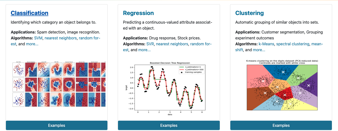
一种典型的无监督学习算法，主要用于将相似的样本自动归到一个类别中。

在聚类算法中根据样本之间的相似性，将样本划分到不同的类别中，对于不同的相似度计算方法，会得到不同的聚类结果，常用的相似度计算方法有欧式距离法。

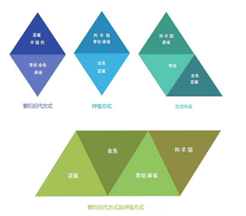
举例
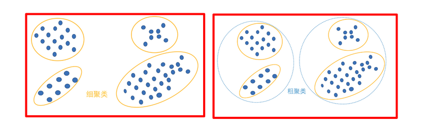
使用不同的聚类准则，会产生的聚类结果不同。

在无监督学习中，数据 = (特征，) 没有标签
以NBA球员詹姆斯的个人统计为例, 根据詹姆斯个人统计来预测骑士队输赢或者个人效率值外，我们还可以对该数据做聚类 (clustering)，即将训练集中的数据分成若干组，每组成为一个簇 (cluster)。

假设聚类方法将数据聚成二个簇 A 和 B，如下图

后来发现簇 A 代表赢，簇 B 代表输。聚类的用处就是可以找到一个潜在的原因来解释为什么样例 1 和 4 可以赢球。难道真的是只要詹姆斯三双就可以赢球？

聚类算法在现实中的应用

• 用户画像，广告推荐，Data Segmentation，搜索引擎的流量推荐，恶意流量识别
• 基于位置信息的商业推送，新闻聚类，筛选排序
• 图像分割，降维，识别；离群点检测；信用卡异常消费；发掘相同功能的基因片段
  

k-means是聚类算法中最典型的算法

聚类算法实现流程

k-means其实包含两层内容：

• K : 初始中心点个数（计划聚类数）
• means：求中心点到其他数据点距离的平均值

k-means聚类步骤

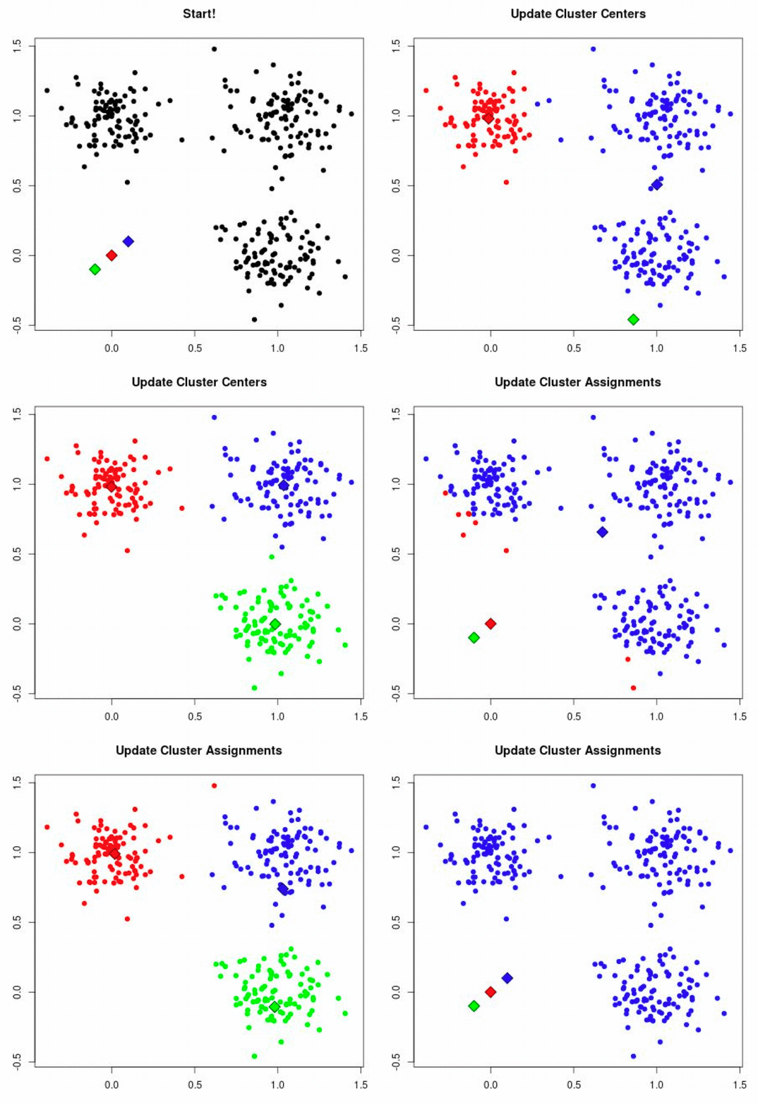
1、随机设置K个特征空间内的点作为初始的聚类中心
2、对于其他每个点计算到K个中心的距离(3个)，未知的点选择最近的一个聚类中心点作为标记类别
3、接着对着标记的聚类中心之后，重新计算出每个聚类的新中心点（平均值）
4、如果计算得出的新中心点与原中心点一样（质心不再移动），那么结束，否则重新进行第二步过程
通过下图解释实现流程：


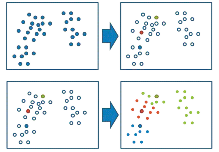
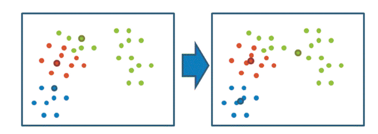
k聚类动态效果图

案例练习

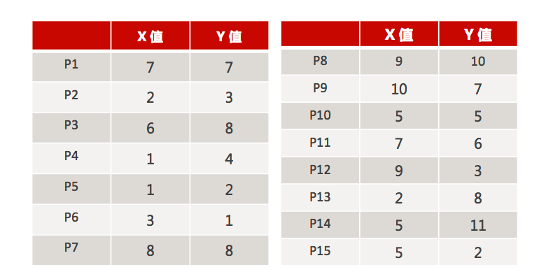
1、随机设置K个特征空间内的点作为初始的聚类中心（本案例中设置p1和p2）

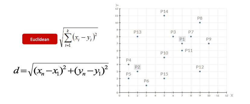
2、对于其他每个点计算到K个中心的距离，未知的点选择最近的一个聚类中心点作为标记类别

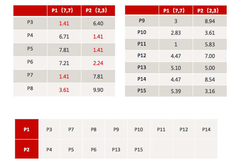
3、接着对着标记的聚类中心之后，重新计算出每个聚类的新中心点（平均值）

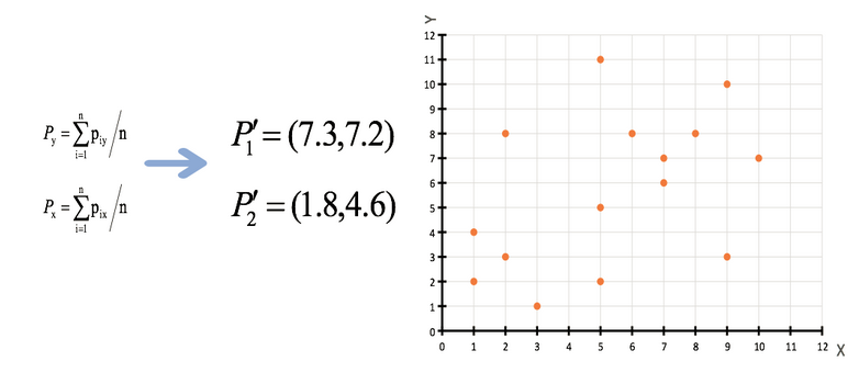
4、如果计算得出的新中心点与原中心点一样（质心不再移动），那么结束，否则重新进行第二步过程【经过判断，需要重复上述步骤，开始新一轮迭代】

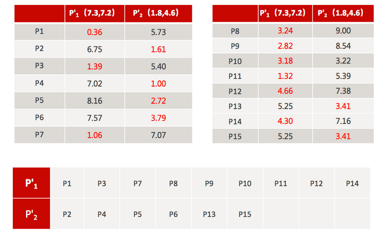
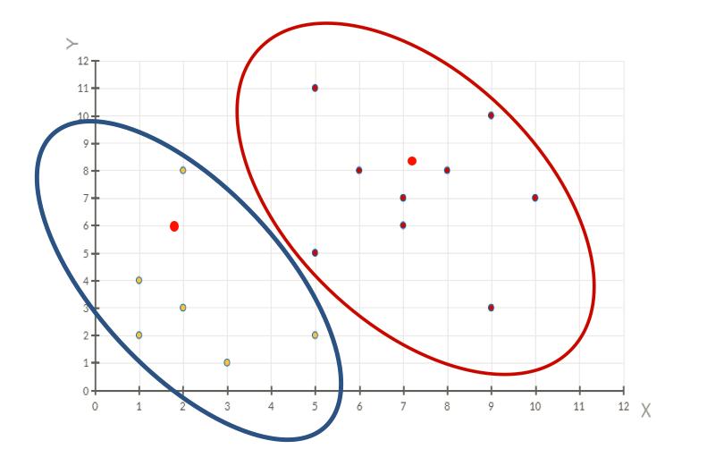
5、当每次迭代结果不变时，认为算法收敛，聚类完成，K-Means一定会停下，不可能陷入一直选质心的过程。

小结

流程:

• 事先确定常数K，常数K意味着最终的聚类类别数;
• 首先随机选定初始点为质心，并通过计算每一个样本与质心之间的相似度(这里为欧式距离)，将样本点归到最相似的类中，
• 接着，重新计算每个类的质心(即为类中心)，重复这样的过程，直到质心不再改变，
• 最终就确定了每个样本所属的类别以及每个类的质心。

注意:

由于每次都要计算所有的样本与每一个质心之间的相似度，故在大规模的数据集上，K-Means算法的收敛速度比较慢

api介绍

sklearn.cluster.KMeans(n_clusters=8)
参数:
n_clusters:开始的聚类中心数量
整型，缺省值=8，生成的聚类数，即产生的质心（centroids）数。
方法:
estimator.fit(x)
estimator.predict(x)
estimator.fit_predict(x)
计算聚类中心并预测每个样本属于哪个类别,相当于先调用fit(x),然后再调用predict(x)

案例实战

import matplotlib.pyplot as plt
from sklearn.cluster import KMeans
from sklearn.datasets import make_blobs
#用calinski_harabaz_score方法评价聚类效果的好坏大概是类间距除以类内距，因此这个值越大越好
from sklearn.metrics import calinski_harabasz_score
# 创建数据
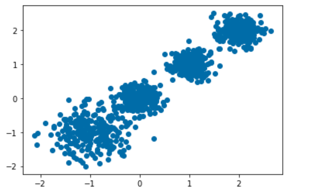
X, y = make_blobs(n_samples=1000, n_features=2, centers=[
[-1, -1], [0, 0], [1, 1], [2, 2]], cluster_std=[0.4, 0.2, 0.2, 0.2], random_state=9)
X.shape, y.shape

((1000, 2), (1000,))

plt.scatter(X[:, 0], X[:, 1])
plt.show()

# kmeans训练,且可视化 聚类=2
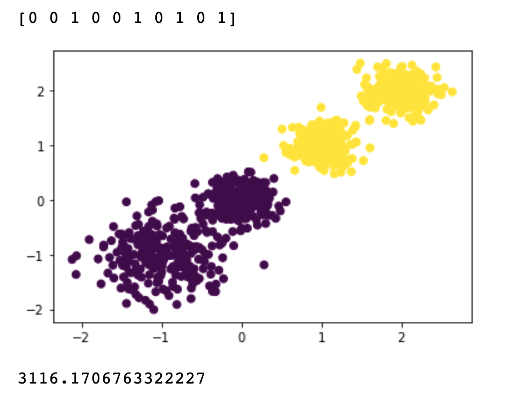
y_predict = KMeans(n_clusters=2, random_state=9).fit_predict(X)
print(y_predict[:10])
plt.scatter(X[:, 0], X[:, 1], c=y_predict)
plt.show()
print(calinski_harabasz_score(X, y_predict))

# kmeans训练,且可视化 聚类=3
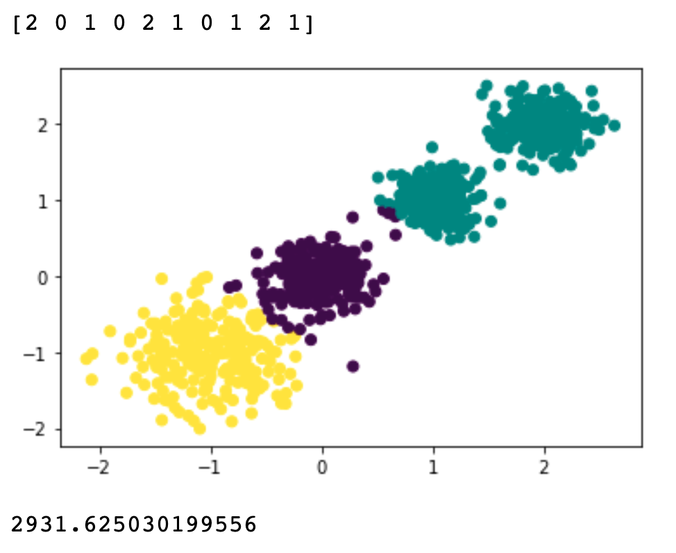
y_predict = KMeans(n_clusters=3, random_state=9).fit_predict(X)
print(y_predict[:10])
plt.scatter(X[:, 0], X[:, 1], c=y_predict)
plt.show()
print(calinski_harabasz_score(X, y_predict))

# kmeans训练,且可视化 聚类=4
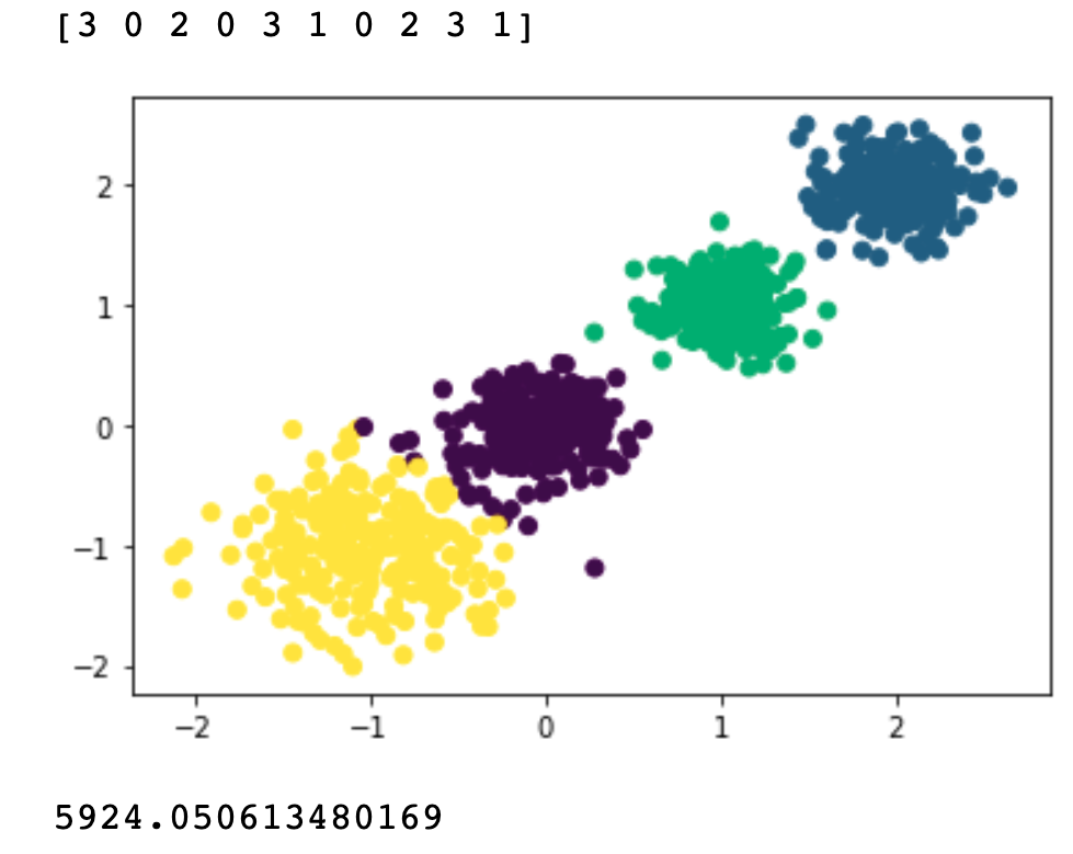
y_predict = KMeans(n_clusters=4, random_state=9).fit_predict(X)
print(y_predict[:10])
plt.scatter(X[:, 0], X[:, 1], c=y_predict)
plt.show()
print(calinski_harabasz_score(X, y_predict))

案例: 探究用户对物品类别的喜好细分

地址: https://www.kaggle.com/c/instacart-market-basket-analysis/data
数据如下：

• order_products__prior.csv：订单与商品信息
  字段：order_id, product_id, add_to_cart_order, reordered
• products.csv：商品信息
  字段：product_id, product_name, aisle_id, department_id
• orders.csv：用户的订单信息
  字段：order_id,user_id,eval_set,order_number,….
• aisles.csv：商品所属具体物品类别
  字段： aisle_id, aisle

1.获取数据

import pandas as pd
from sklearn.decomposition import PCA
from sklearn.cluster import KMeans
## 轮廓系数取值为[-1, 1]，其值越大越好，且当值为负时，
# 表明样本被分配到错误的簇中，聚类结果不可接受。对于接近0的结果，则表明聚类结果有重叠的情况
from sklearn.metrics import silhouette_score
# 1.获取数据
order_product = pd.read_csv("./data/instacart/order_products__prior.csv")
products = pd.read_csv("./data/instacart/products.csv")
orders = pd.read_csv("./data/instacart/orders.csv")
aisles = pd.read_csv("./data/instacart/aisles.csv")

order_product.head()

	order_id	product_id	add_to_cart_order	reordered
0	2	33120	1	1
1	2	28985	2	1
2	2	9327	3	0
3	2	45918	4	1
4	2	30035	5	0

products.head()

	product_id	product_name	aisle_id	department_id
0	1	Chocolate Sandwich Cookies	61	19
1	2	All-Seasons Salt	104	13
2	3	Robust Golden Unsweetened Oolong Tea	94	7
3	4	Smart Ones Classic Favorites Mini Rigatoni Wit...	38	1
4	5	Green Chile Anytime Sauce	5	13

orders.head()

	order_id	user_id	eval_set	order_number	order_dow	order_hour_of_day	days_since_prior_order
0	2539329	1	prior	1	2	8	NaN
1	2398795	1	prior	2	3	7	15.0
2	473747	1	prior	3	3	12	21.0
3	2254736	1	prior	4	4	7	29.0
4	431534	1	prior	5	4	15	28.0

aisles.head()

	aisle_id	aisle
0	1	prepared soups salads
1	2	specialty cheeses
2	3	energy granola bars
3	4	instant foods
4	5	marinades meat preparation

2.数据基本处理

# 合并表格
table1 = pd.merge(order_product, products, on=["product_id", "product_id"])
table2 = pd.merge(table1, orders, on=["order_id", "order_id"])
table = pd.merge(table2, aisles, on=["aisle_id", "aisle_id"])
print(table.shape)

(32434489, 14)

table.head()

	order_id	product_id	add_to_cart_order	reordered	product_name	aisle_id	department_id	user_id	eval_set	order_number	order_dow	order_hour_of_day	days_since_prior_order	aisle
0	2	33120	1	1	Organic Egg Whites	86	16	202279	prior	3	5	9	8.0	eggs
1	26	33120	5	0	Organic Egg Whites	86	16	153404	prior	2	0	16	7.0	eggs
2	120	33120	13	0	Organic Egg Whites	86	16	23750	prior	11	6	8	10.0	eggs
3	327	33120	5	1	Organic Egg Whites	86	16	58707	prior	21	6	9	8.0	eggs
4	390	33120	28	1	Organic Egg Whites	86	16	166654	prior	48	0	12	9.0	eggs

# 交叉表合并  table["user_id"]为行索引, table["aisle"]为列索引
data = pd.crosstab(table["user_id"], table["aisle"])
data.head()

aisle	air fresheners candles	asian foods	baby accessories	baby bath body care	baby food formula	bakery desserts	baking ingredients	baking supplies decor	beauty	beers coolers	...	spreads	tea	tofu meat alternatives	tortillas flat bread	trail mix snack mix	trash bags liners	vitamins supplements	water seltzer sparkling water	white wines	yogurt
user_id
1	0	0	0	0	0	0	0	0	0	0	...	1	0	0	0	0	0	0	0	0	1
2	0	3	0	0	0	0	2	0	0	0	...	3	1	1	0	0	0	0	2	0	42
3	0	0	0	0	0	0	0	0	0	0	...	4	1	0	0	0	0	0	2	0	0
4	0	0	0	0	0	0	0	0	0	0	...	0	0	0	1	0	0	0	1	0	0
5	0	2	0	0	0	0	0	0	0	0	...	0	0	0	0	0	0	0	0	0	3

5 rows × 134 columns

data.shape

(206209, 134)

#  数据截取
new_data = data[:1000]
# 3.特征工程 — pca
transfer = PCA(0.9)
trans_data = transfer.fit_transform(new_data)
trans_data.shape

(1000, 22)

# 4.机器学习（k-means）
estimator = KMeans(n_clusters=5)
y_pred = estimator.fit_predict(trans_data)
print(y_pred[:20])
# 5.模型评估
print(silhouette_score(trans_data, y_pred))

[3 0 3 3 3 3 0 3 3 0 3 3 3 3 3 3 3 3 3 3]
0.4585956252548508

2D数据类别划分

任务:

1、采用Kmeans算法实现2D数据自动聚类，预测V1=80,V2=60数据类别；

2、计算预测准确率，完成结果矫正

3、采用KNN、Meanshift算法，重复步骤1-2
Mean Shift算法,一般是指一个迭代的步骤,即先算出当前点的偏移均值,移动该点到其偏移均值,然后以此为新的起始点,继续移动,直到满足一定的条件结束
数据：data.csv

#load the data
import pandas as pd
import numpy as np
data = pd.read_csv('data.csv')
data.head()

	V1	V2	labels
0	2.072345	-3.241693	0
1	17.936710	15.784810	0
2	1.083576	7.319176	0
3	11.120670	14.406780	0
4	23.711550	2.557729	0

#define X and y
X = data.drop(['labels'],axis=1)
y = data.loc[:,'labels']
y.head()

0    0
1    0
2    0
3    0
4    0
Name: labels, dtype: int64

pd.value_counts(y)

2    1156
1     954
0     890
Name: labels, dtype: int64

%matplotlib inline
from matplotlib import pyplot as plt
fig1 = plt.figure()
plt.scatter(X.loc[:,'V1'],X.loc[:,'V2'])
plt.title("un-labled data")
plt.xlabel('V1')
plt.ylabel('V2')
plt.show()

fig1 = plt.figure()
label0 = plt.scatter(X.loc[:,'V1'][y==0],X.loc[:,'V2'][y==0])
label1 = plt.scatter(X.loc[:,'V1'][y==1],X.loc[:,'V2'][y==1])
label2 = plt.scatter(X.loc[:,'V1'][y==2],X.loc[:,'V2'][y==2])

plt.title("labled data")
plt.xlabel('V1')
plt.ylabel('V2'))
plt.legend((label0,label1,label2),('label0','label1','label2'))
plt.show()

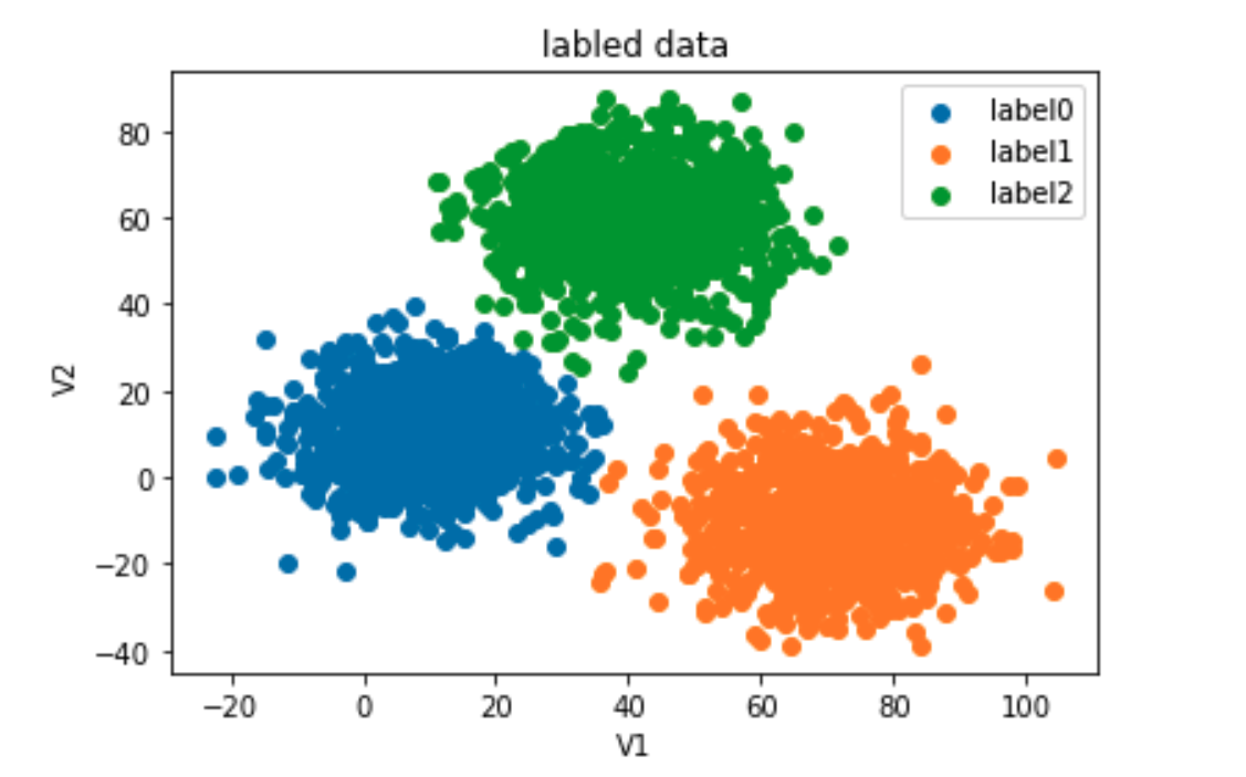
print(X.shape,y.shape)

(3000, 2) (3000,)

from sklearn.cluster import KMeans
KM = KMeans(n_clusters=3, random_state=0)
KM.fit(X)

KMeans(n_clusters=3, random_state=0)

centers = KM.cluster_centers_
centers # 3个中心坐标

array([[ 69.92418447, -10.11964119],
       [ 40.68362784,  59.71589274],
       [  9.4780459 ,  10.686052  ]])

fig1 = plt.figure()
label0 = plt.scatter(X.loc[:,'V1'][y==0],X.loc[:,'V2'][y==0])
label1 = plt.scatter(X.loc[:,'V1'][y==1],X.loc[:,'V2'][y==1])
label2 = plt.scatter(X.loc[:,'V1'][y==2],X.loc[:,'V2'][y==2])
plt.title("labled data")
plt.xlabel('V1')
plt.ylabel('V2')
# 画中心点
plt.scatter(centers[:, 0], centers[:, 1])
plt.legend((label0,label1,label2),('label0','label1','label2'))
plt.show()

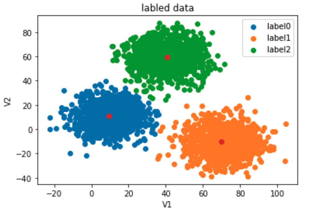
# 预测V1=80,V2=60数据类别；
y_predict = KM.predict(np.array([[80, 60]]))
y_predict

array([1], dtype=int32)

y_predict = KM.predict(X)
print(pd.value_counts(y_predict))

1    1149
0     952
2     899
dtype: int64

pd.value_counts(y)

2    1156
1     954
0     890
Name: labels, dtype: int64

from sklearn.metrics import accuracy_score
accuracy_score(y, y_predict)

0.0023333333333333335

#visualize the data and results
fig4 = plt.subplot(121)
label0 = plt.scatter(X.loc[:,'V1'][y_predict==0],X.loc[:,'V2'][y_predict==0])
label1 = plt.scatter(X.loc[:,'V1'][y_predict==1],X.loc[:,'V2'][y_predict==1])
label2 = plt.scatter(X.loc[:,'V1'][y_predict==2],X.loc[:,'V2'][y_predict==2])

plt.title("predicted data")
plt.xlabel('V1')
plt.ylabel('V2')
plt.legend((label0,label1,label2),('label0','label1','label2'))
plt.scatter(centers[:,0],centers[:,1])

fig5 = plt.subplot(122)
label0 = plt.scatter(X.loc[:,'V1'][y==0],X.loc[:,'V2'][y==0])
label1 = plt.scatter(X.loc[:,'V1'][y==1],X.loc[:,'V2'][y==1])
label2 = plt.scatter(X.loc[:,'V1'][y==2],X.loc[:,'V2'][y==2])

plt.title("labled data")
plt.xlabel('V1')
plt.ylabel('V2')
plt.legend((label0,label1,label2),('label0','label1','label2'))
plt.scatter(centers[:,0],centers[:,1])
plt.show()

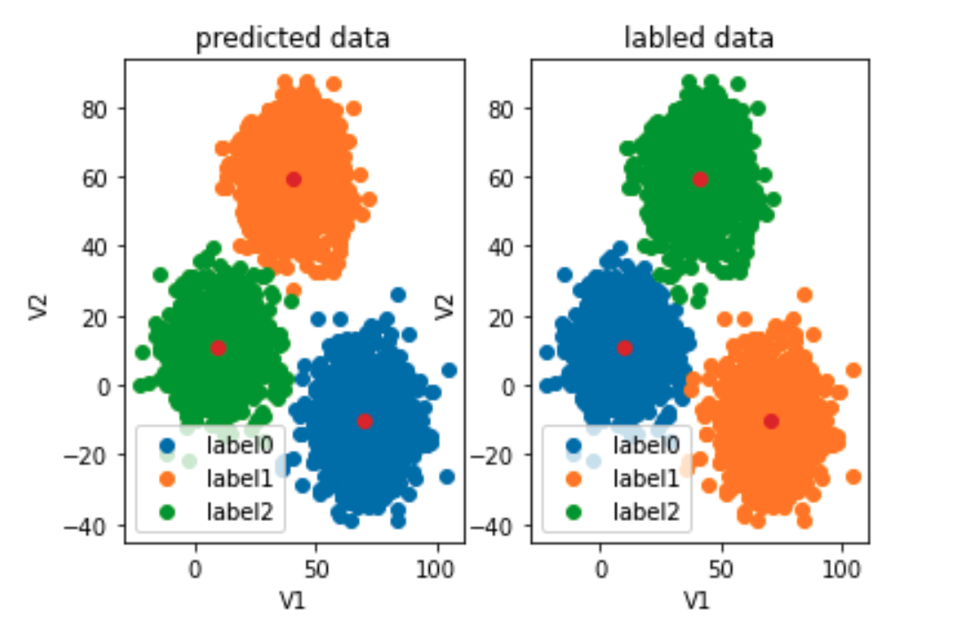
#correct the results
y_corrected = []
for i in y_predict:
    if i == 0:
        y_corrected.append(1)
    elif i == 1:
        y_corrected.append(2)
    else:
        y_corrected.append(0)
y_corrected = np.array(y_corrected)

accuracy_score(y, y_corrected)

0.997

#visualize the data and results
fig4 = plt.subplot(121)
label0 = plt.scatter(X.loc[:,'V1'][y_corrected==0],X.loc[:,'V2'][y_corrected==0])
label1 = plt.scatter(X.loc[:,'V1'][y_corrected==1],X.loc[:,'V2'][y_corrected==1])
label2 = plt.scatter(X.loc[:,'V1'][y_corrected==2],X.loc[:,'V2'][y_corrected==2])

plt.title("predicted data")
plt.xlabel('V1')
plt.ylabel('V2')
plt.legend((label0,label1,label2),('label0','label1','label2'))
plt.scatter(centers[:,0],centers[:,1])

fig5 = plt.subplot(122)
label0 = plt.scatter(X.loc[:,'V1'][y==0],X.loc[:,'V2'][y==0])
label1 = plt.scatter(X.loc[:,'V1'][y==1],X.loc[:,'V2'][y==1])
label2 = plt.scatter(X.loc[:,'V1'][y==2],X.loc[:,'V2'][y==2])

plt.title("labled data")
plt.xlabel('V1')
plt.ylabel('V2')
plt.legend((label0,label1,label2),('label0','label1','label2'))
plt.scatter(centers[:,0],centers[:,1])
plt.show()

注意和KNN 的区别

from sklearn.neighbors import KNeighborsClassifier
KNN = KNeighborsClassifier(n_neighbors=3)
KNN.fit(X,y)

KNeighborsClassifier(n_neighbors=3)

#predict based on the test data V1=80, V2=60
y_predict_knn_test = KNN.predict([[80,60]])
y_predict_knn = KNN.predict(X)
print(y_predict_knn_test)
print('knn accuracy:',accuracy_score(y,y_predict_knn))

[2]
knn accuracy: 1.0

print(pd.value_counts(y_predict_knn),pd.value_counts(y))

2    1156
1     954
0     890
dtype: int64 2    1156
1     954
0     890
Name: labels, dtype: int64

fig6 = plt.subplot(121)
label0 = plt.scatter(X.loc[:,'V1'][y_predict_knn==0],X.loc[:,'V2'][y_predict_knn==0])
label1 = plt.scatter(X.loc[:,'V1'][y_predict_knn==1],X.loc[:,'V2'][y_predict_knn==1])
label2 = plt.scatter(X.loc[:,'V1'][y_predict_knn==2],X.loc[:,'V2'][y_predict_knn==2])

plt.title("knn results")
plt.xlabel('V1')
plt.ylabel('V2')
plt.legend((label0,label1,label2),('label0','label1','label2'))
plt.scatter(centers[:,0],centers[:,1])

fig7 = plt.subplot(122)
label0 = plt.scatter(X.loc[:,'V1'][y==0],X.loc[:,'V2'][y==0])
label1 = plt.scatter(X.loc[:,'V1'][y==1],X.loc[:,'V2'][y==1])
label2 = plt.scatter(X.loc[:,'V1'][y==2],X.loc[:,'V2'][y==2])

plt.title("labled data")
plt.xlabel('V1')
plt.ylabel('V2')
plt.legend((label0,label1,label2),('label0','label1','label2'))
plt.scatter(centers[:,0],centers[:,1])
plt.show()

meanshift

from sklearn.cluster import MeanShift,estimate_bandwidth
# 预估带宽
bw = estimate_bandwidth(X,n_samples=500)

#establish the meanshift model-un-supervised model
ms = MeanShift(bandwidth=bw)
ms.fit(X)

MeanShift(bandwidth=30.84663454820215)

y_predict_ms = ms.predict(X)
print(pd.value_counts(y_predict_ms),pd.value_counts(y))

0    1149
1     952
2     899
dtype: int64 2    1156
1     954
0     890
Name: labels, dtype: int64

#新增代码 打印使用meanshift算法获取的聚类中心 与kmeans算法对比 中心点非常接近
centers2 = ms.cluster_centers_
print(centers2)#meanshift聚类中心

[[ 40.60158864  59.65137971]
 [ 70.01854306 -10.11803404]
 [  9.56752568  10.79316266]]

centers

array([[ 69.92418447, -10.11964119],
       [ 40.68362784,  59.71589274],
       [  9.4780459 ,  10.686052  ]])

fig6 = plt.subplot(121)
label0 = plt.scatter(X.loc[:,'V1'][y_predict_ms==0],X.loc[:,'V2'][y_predict_ms==0])
label1 = plt.scatter(X.loc[:,'V1'][y_predict_ms==1],X.loc[:,'V2'][y_predict_ms==1])
label2 = plt.scatter(X.loc[:,'V1'][y_predict_ms==2],X.loc[:,'V2'][y_predict_ms==2])

plt.title("ms results")
plt.xlabel('V1')
plt.ylabel('V2')
plt.legend((label0,label1,label2),('label0','label1','label2'))
plt.scatter(centers[:,0],centers[:,1])

fig7 = plt.subplot(122)
label0 = plt.scatter(X.loc[:,'V1'][y==0],X.loc[:,'V2'][y==0])
label1 = plt.scatter(X.loc[:,'V1'][y==1],X.loc[:,'V2'][y==1])
label2 = plt.scatter(X.loc[:,'V1'][y==2],X.loc[:,'V2'][y==2])

plt.title("labled data")
plt.xlabel('V1')
plt.ylabel('V2')
plt.legend((label0,label1,label2),('label0','label1','label2'))
plt.scatter(centers[:,0],centers[:,1])
plt.show()

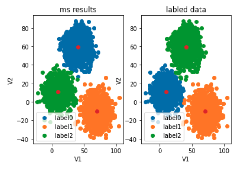
#correct the results
y_corrected_ms = []
for i in y_predict_ms:
    if i==0:
        y_corrected_ms.append(2)
    elif i==1:
        y_corrected_ms.append(1)
    else:
        y_corrected_ms.append(0)
y_corrected_ms = np.array(y_corrected_ms)
print(type(y_corrected_ms))
print(pd.value_counts(y_corrected_ms),pd.value_counts(y))

<class 'numpy.ndarray'>
2    1149
1     952
0     899
dtype: int64 2    1156
1     954
0     890
Name: labels, dtype: int64

fig6 = plt.subplot(121)
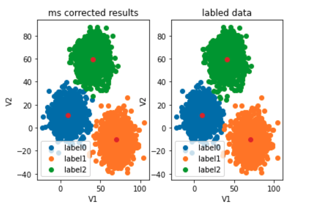
label0 = plt.scatter(X.loc[:,'V1'][y_corrected_ms==0],X.loc[:,'V2'][y_corrected_ms==0])
label1 = plt.scatter(X.loc[:,'V1'][y_corrected_ms==1],X.loc[:,'V2'][y_corrected_ms==1])
label2 = plt.scatter(X.loc[:,'V1'][y_corrected_ms==2],X.loc[:,'V2'][y_corrected_ms==2])

plt.title("ms corrected results")
plt.xlabel('V1')
plt.ylabel('V2')
plt.legend((label0,label1,label2),('label0','label1','label2'))
plt.scatter(centers[:,0],centers[:,1])

fig7 = plt.subplot(122)
label0 = plt.scatter(X.loc[:,'V1'][y==0],X.loc[:,'V2'][y==0])
label1 = plt.scatter(X.loc[:,'V1'][y==1],X.loc[:,'V2'][y==1])
label2 = plt.scatter(X.loc[:,'V1'][y==2],X.loc[:,'V2'][y==2])

plt.title("labled data")
plt.xlabel('V1')
plt.ylabel('V2')
plt.legend((label0,label1,label2),('label0','label1','label2'))
plt.scatter(centers[:,0],centers[:,1])
plt.show()

Meanshift

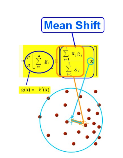
一般是指一个迭代的步骤,即先算出当前点的偏移均值,移动该点到其偏移均值,然后以此为新的起始点,继续移动,直到满足一定的条件结束.

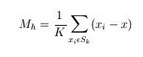
Sk是一个半径为h的高维球区域,满足以下关系的y点的集合,

k表示在这n个样本点xi中,有k个点落入Sk区域中.

以上是官方的说法，在d维空间中，任选一个点，然后以这个点为圆心，h为半径做一个高维球，因为有d维，d可能大于2，所以是高维球。落在这个球内的所有点和圆心都会产生一个向量，向量是以圆心为起点落在球内的点位终点。然后把这些向量都相加。相加的结果就是Meanshift向量。

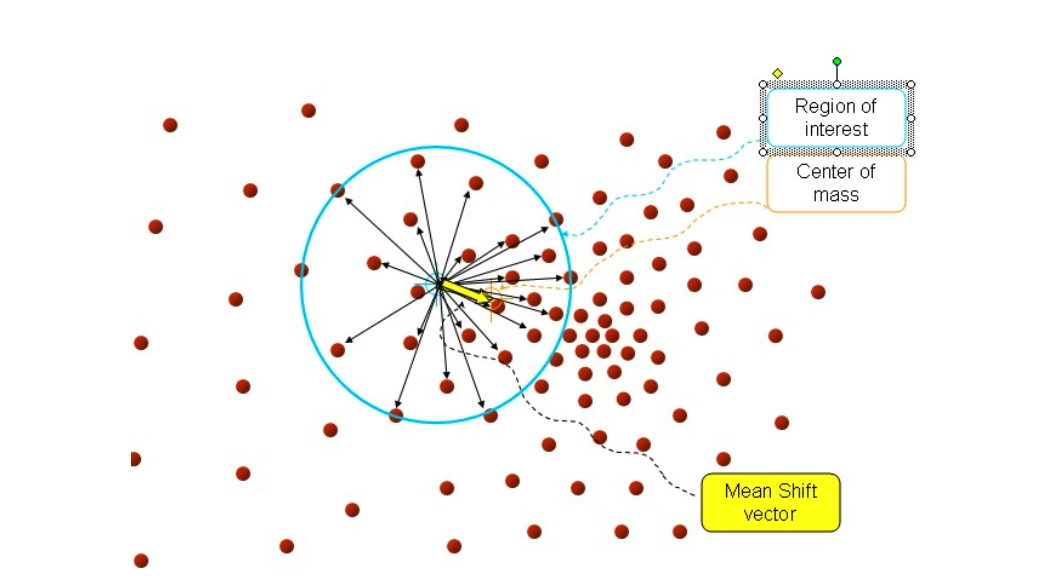
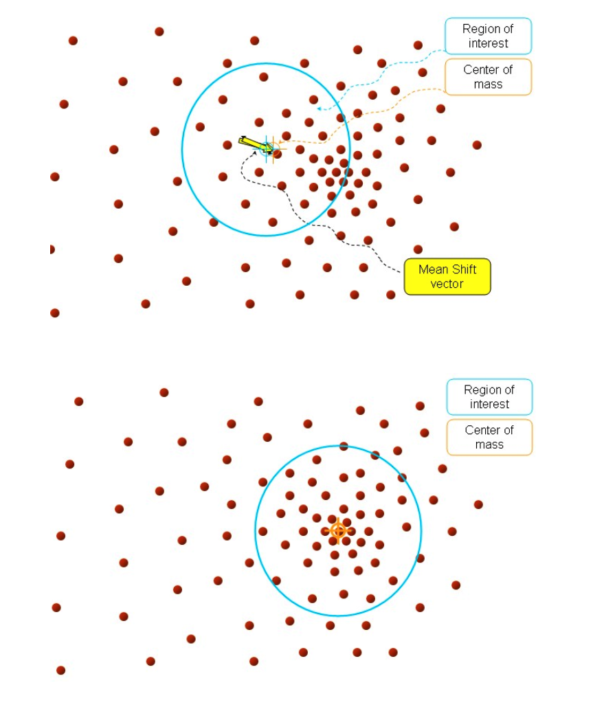
再以meanshift向量的终点为圆心，再做一个高维的球。如下图所以，重复以上步骤，就可得到一个meanshift向量。如此重复下去，meanshift算法可以收敛到概率密度最大得地方。也就是最稠密的地方。

mean shift 聚类流程：

假设在一个多维空间中有很多数据点需要进行聚类，Mean Shift的过程如下：

1. 在未被标记的数据点中随机选择一个点作为中心center；
2. 找出离center距离在bandwidth之内的所有点，记做集合M，认为这些点属于簇c。同时，把这些球内点属于这个类的概率加1，这个参数将用于最后步骤的分类
3. 以center为中心点，计算从center开始到集合M中每个元素的向量，将这些向量相加，得到向量shift。
4. center = center+shift。即center沿着shift的方向移动，移动距离是||shift||。
5. 重复步骤2、3、4，直到shift的大小很小（就是迭代到收敛），记住此时的center。注意，这个迭代过程中遇到的点都应该归类到簇c。
6. 如果收敛时当前簇c的center与其它已经存在的簇c2中心的距离小于阈值，那么把c2和c合并。否则，把c作为新的聚类，增加1类。 重复1、2、3、4、5直到所有的点都被标记访问。
7. 分类：根据每个类，对每个点的访问频率，取访问频率最大的那个类，作为当前点集的所属类。 简单的说，mean shift就是沿着密度上升的方向寻找同属一个簇的数据点。
   

使用MeanShift

from sklearn.cluster import MeanShift, estimate_bandwidth
bw = estimate_bandwidth(X, n_samples=500)
print('bw = ', bw)
ms = MeanShift(bandwidth=bw)
ms.fit(X)
y_predict_ms = ms.predict(X)
centers = ms.cluster_centers_
print(centers)

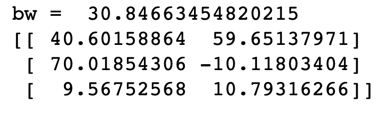
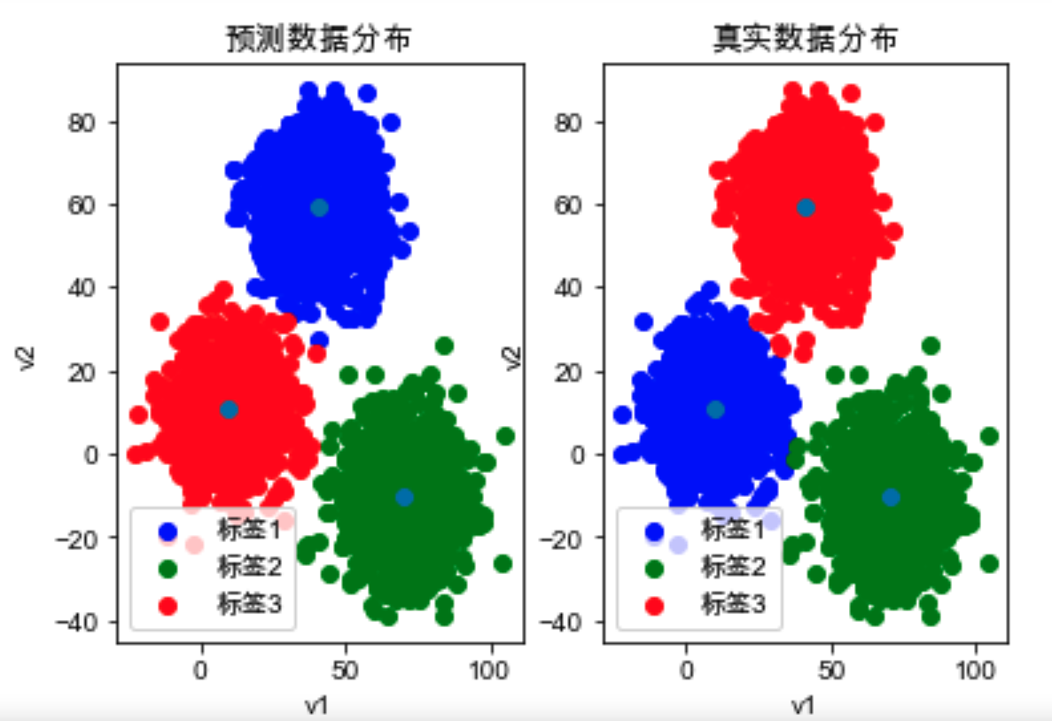
fig1 = plt.subplot(121)
label0 = plt.scatter(X.loc[:, 'V1'][y_predict_ms==0], X.loc[:, 'V2'][y_predict_ms==0], color='b' )
label1 = plt.scatter(X.loc[:, 'V1'][y_predict_ms==1], X.loc[:, 'V2'][y_predict_ms==1], color='g')
label2 = plt.scatter(X.loc[:, 'V1'][y_predict_ms==2], X.loc[:, 'V2'][y_predict_ms==2], color='r')
plt.title("预测数据分布")
plt.xlabel('v1')
plt.ylabel('v2')
plt.legend((label0,label1,label2), ('标签1', '标签2','标签3'))
plt.scatter(centers[:, 0], centers[:, 1])
plt.subplot(122)
label0 = plt.scatter(X.loc[:, 'V1'][y==0], X.loc[:, 'V2'][y==0], color='b' )
label1 = plt.scatter(X.loc[:, 'V1'][y==1], X.loc[:, 'V2'][y==1], color='g')
label2 = plt.scatter(X.loc[:, 'V1'][y==2], X.loc[:, 'V2'][y==2], color='r')
plt.title("真实数据分布")
plt.xlabel('v1')
plt.ylabel('v2')
plt.legend((label0,label1,label2), ('标签1', '标签2','标签3'))
plt.scatter(centers[:, 0], centers[:, 1])

plt.show()

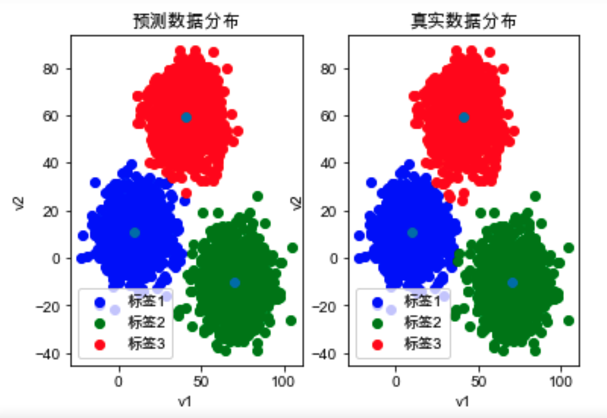
#correct the results
y_corrected_ms = []
for i in y_predict_ms:
    if i==0:
        y_corrected_ms.append(2)
    elif i==1:
        y_corrected_ms.append(1)
    else:
        y_corrected_ms.append(0)
print(pd.value_counts(y_corrected_ms),pd.value_counts(y))
y_predict = np.array(y_corrected_ms)
fig1 = plt.subplot(121)
label0 = plt.scatter(X.loc[:, 'V1'][y_predict==0], X.loc[:, 'V2'][y_predict==0], color='b' )
label1 = plt.scatter(X.loc[:, 'V1'][y_predict==1], X.loc[:, 'V2'][y_predict==1], color='g')
label2 = plt.scatter(X.loc[:, 'V1'][y_predict==2], X.loc[:, 'V2'][y_predict==2], color='r')
plt.title("预测数据分布")
plt.xlabel('v1')
plt.ylabel('v2')
plt.legend((label0,label1,label2), ('标签1', '标签2','标签3'))
plt.scatter(centers[:, 0], centers[:, 1])
plt.subplot(122)
label0 = plt.scatter(X.loc[:, 'V1'][y==0], X.loc[:, 'V2'][y==0], color='b' )
label1 = plt.scatter(X.loc[:, 'V1'][y==1], X.loc[:, 'V2'][y==1], color='g')
label2 = plt.scatter(X.loc[:, 'V1'][y==2], X.loc[:, 'V2'][y==2], color='r')
plt.title("真实数据分布")
plt.xlabel('v1')
plt.ylabel('v2')
plt.legend((label0,label1,label2), ('标签1', '标签2','标签3'))
plt.scatter(centers[:, 0], centers[:, 1])

plt.show()

实现

import random
from sklearn import datasets
import numpy as np
import matplotlib.pyplot as plt
from mpl_toolkits.mplot3d import Axes3D
class Kmeans():
    """Kmeans聚类算法.

    Parameters:
    -----------
    k: int
        聚类的数目.
    max_iterations: int
        最大迭代次数.
    varepsilon: float
        判断是否收敛, 如果上一次的所有k个聚类中心与本次的所有k个聚类中心的差都小于varepsilon,
        则说明算法已经收敛
    """
    def __init__(self, k=2, max_iterations=500, varepsilon=1e-4):
        self.k = k
        self.max_iterations = max_iterations
        self.varepsilon = varepsilon

    # 从所有样本中随机选取self.k样本作为初始的聚类中心
    def init_random_centroids(self, X):
        n_samples, n_features = np.shape(X)
        centroids = np.zeros((self.k, n_features))
        for i in range(self.k):
            centroid = X[np.random.choice(range(n_samples))]
            centroids[i] = centroid
        return centroids

    # 返回距离该样本最近的一个中心索引[0, self.k)
    def _closest_centroid(self, sample, centroids):
        distances = self.euclidean_distance(sample, centroids)
        closest_i = np.argmin(distances)
        return closest_i

    # 将所有样本进行归类，归类规则就是将该样本归类到与其最近的中心
    def create_clusters(self, centroids, X):
        n_samples = np.shape(X)[0]
        clusters = [[] for _ in range(self.k)]
        for sample_i, sample in enumerate(X):
            centroid_i = self._closest_centroid(sample, centroids)
            clusters[centroid_i].append(sample_i)
        return clusters

    # 对中心进行更新
    def update_centroids(self, clusters, X):
        n_features = np.shape(X)[1]
        centroids = np.zeros((self.k, n_features))
        for i, cluster in enumerate(clusters):
            centroid = np.mean(X[cluster], axis=0)
            centroids[i] = centroid
        return centroids

    # 将所有样本进行归类，其所在的类别的索引就是其类别标签
    def get_cluster_labels(self, clusters, X):
        y_pred = np.zeros(np.shape(X)[0])
        for cluster_i, cluster in enumerate(clusters):
            for sample_i in cluster:
                y_pred[sample_i] = cluster_i
        return y_pred

    # 计算一个样本与数据集中所有样本的欧氏距离的平方
    def euclidean_distance(self, one_sample, X):
        one_sample = one_sample.reshape(1, -1)
        X = X.reshape(X.shape[0], -1)
        distances = np.power(np.tile(one_sample, (X.shape[0], 1)) - X, 2).sum(axis=1)
        return distances

    # 对整个数据集X进行Kmeans聚类，返回其聚类的标签
    def predict(self, X):
        # 从所有样本中随机选取self.k样本作为初始的聚类中心
        centroids = self.init_random_centroids(X)

        # 迭代，直到算法收敛(上一次的聚类中心和这一次的聚类中心几乎重合)或者达到最大迭代次数
        for _ in range(self.max_iterations):
            # 将所有进行归类，归类规则就是将该样本归类到与其最近的中心
            clusters = self.create_clusters(centroids, X)
            former_centroids = centroids

            # 计算新的聚类中心
            centroids = self.update_centroids(clusters, X)

            # 如果聚类中心几乎没有变化，说明算法已经收敛，退出迭代
            diff = centroids - former_centroids
            if diff.any() < self.varepsilon:
                break

        return self.get_cluster_labels(clusters, X)


def main():
    # Load the dataset
    X, y = datasets.make_blobs(n_samples=10000,
                               n_features=3,
                               centers=[[3,3, 3], [0,0,0], [1,1,1], [2,2,2]],
                               cluster_std=[0.2, 0.1, 0.2, 0.2],
                               random_state =9)

    # 用Kmeans算法进行聚类
    clf = Kmeans(k=4)
    y_pred = clf.predict(X)
    print(y_pred)

    # 可视化聚类效果
    # fig = plt.figure(figsize=(12, 8))
    # ax = Axes3D(fig, rect=[0, 0, 1, 1], elev=30, azim=20)
    # plt.scatter(X[y==0][:, 0], X[y==0][:, 1], X[y==0][:, 2])
    # plt.scatter(X[y==1][:, 0], X[y==1][:, 1], X[y==1][:, 2])
    # plt.scatter(X[y==2][:, 0], X[y==2][:, 1], X[y==2][:, 2])
    # plt.scatter(X[y==3][:, 0], X[y==3][:, 1], X[y==3][:, 2])
    # plt.show()

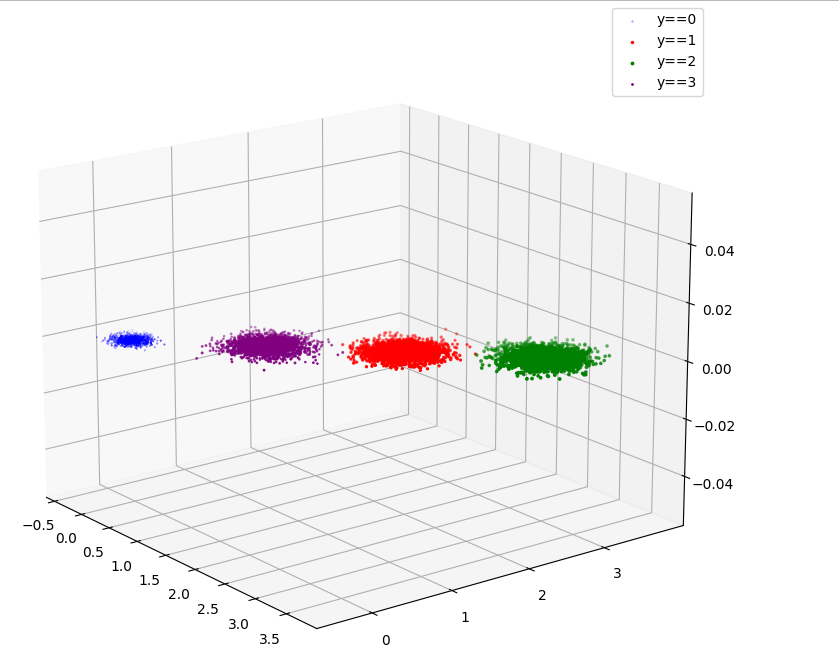
    fig = plt.figure(figsize=(12, 8))
    ax = Axes3D(fig)
    plt.scatter(X[y_pred==0][:, 0], X[y_pred==0][:, 1], X[y_pred==0][:, 2], label='y==0', color='b')
    plt.scatter(X[y_pred==1][:, 0], X[y_pred==1][:, 1], X[y_pred==1][:, 2], label='y==1', color='r')
    plt.scatter(X[y_pred==2][:, 0], X[y_pred==2][:, 1], X[y_pred==2][:, 2], label='y==2', color='g')
    plt.scatter(X[y_pred==3][:, 0], X[y_pred==3][:, 1], X[y_pred==3][:, 2], label='y==3', color='purple')
    plt.legend()
    plt.show()

if __name__ == "__main__":
    main()

实验结果