机器人学-轨迹规划
机器人学-轨迹规划
轨迹规划的概念
轨迹:指的是操作臂每个自由度的位置、速度和加速度的时间历程。
机器人的轨迹规划是指:已知作业任务的要求,在笛卡儿空间或者关节空间内规划出机器人末端的运行轨迹,也就是要建立机器人在运动过程 中时间与空间的函数关系,在轨迹规划上,还要考虑到机器人的性能。所以,工业机器人的轨迹规划一般表示为位移、速度、加速度等运动量关于时间的函数,该函数可以精确地描述工业机器人在任意时间的位置信息和姿态信息。
关节角度空间以及笛卡尔空间
| 维度 | 关节角度空间 | 笛卡尔工作空间 |
|---|---|---|
| 描述对象 | 机器人关节的角度 / 位移 | 机器人末端的位置 + 姿态 |
| 空间维度 | 等于机器人的关节数(如 6 轴→6 维) | 6 维(3 位置 + 3 姿态) |
| 规划逻辑 | 直接给关节角度指令 | 先给末端位姿,再转成关节角度 |
| 计算复杂度 | 低(无需逆运动学) | 高(需逆运动学、奇异点处理) |
| 轨迹可见性 | 末端轨迹不可见 | 末端轨迹直观可控 |
笛卡儿空间轨迹规划的对象一般是工业机器人末端执行器的运动量,如位移、速度、加速度等,这些运动量可以直观清楚地反映出机器人末端执行器的运动情况。但是, 一般还需要通过求运动学逆解来得到机器人关节的运动信息,才可作为机器人运动的输入量 。
关节空间轨迹规划是指在机器人或运动系统的关节空间中规划运动轨迹,即确定各个关节角度随时间的变化,以实现所需的运动任务。相比于笛卡儿空间轨迹规划,关节空间轨迹规划更加直接,能够更精确地控制机器人的运动。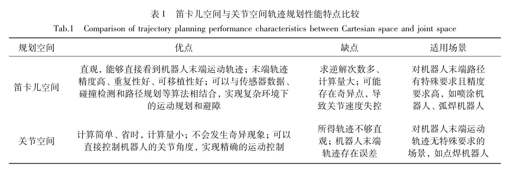
直线插值
是最基础的插值方法,核心逻辑是在两个离散点之间生成一条 “直线”,中间点的取值与时间(或步长)呈线性关系。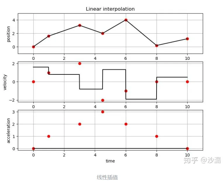
红圈内为给定的中间点值,黑色实线为插值的结果。
关节空间规划方法
插值是轨迹规划的核心技术,本质是在离散的起始点和目标点之间生成连续、平滑的中间过渡点,让机器人的运动从 “跳跃式” 变成 “连续式”。
三次多项式: 用三次多项式拟合关节角度,保证起点和终点的位置、速度连续。
θ(t)=a0+a1t+a2t2+a3t3\theta(t) = a_0 + a_1 t + a_2 t^2 + a_3 t^3θ(t)=a0+a1t+a2t2+a3t3
起始条件:
θ(0)=θ0,θ˙(0)=0\theta(0) = \theta_0, \quad \dot{\theta}(0) = 0θ(0)=θ0,θ˙(0)=0
终止条件:
θ(tf)=θf,θ˙(tf)=0\theta(t_f) = \theta_f, \quad \dot{\theta}(t_f) = 0θ(tf)=θf,θ˙(tf)=0
位置、速度以及加速度为:
θ(t)=a0+a1t+a2t2+a3t3\theta(t) = a_0 + a_1 t + a_2 t^2 + a_3 t^3θ(t)=a0+a1t+a2t2+a3t3
θ˙(t)=a1+2a2t+3a3t2\dot{\theta}(t) = a_1 + 2a_2 t + 3a_3 t^2θ˙(t)=a1+2a2t+3a3t2
θ¨(t)=2a2+6a3t\ddot{\theta}(t) = 2a_2 + 6a_3 tθ¨(t)=2a2+6a3t
代入可得
θ0=a0θf=a0+a1tf+a2tf2+a3tf30=a10=a1+2a2tf+3a3tf2\theta_0 = a_0 \\ \theta_f = a_0 + a_1 t_f + a_2 t_f^2 + a_3 t_f^3 \\ 0 = a_1 \\ 0 = a_1 + 2a_2 t_f + 3a_3 t_f^2θ0=a0θf=a0+a1tf+a2tf2+a3tf30=a10=a1+2a2tf+3a3tf2
最终系数为:
a0=θ0a1=0a2=3tf2(θf−θ0)a3=−2tf3(θf−θ0)a_0 = \theta_0 \\ a_1 = 0 \\ a_2 = \dfrac{3}{t_f^2} \left( \theta_f - \theta_0 \right) \\ a_3 = -\dfrac{2}{t_f^3} \left( \theta_f - \theta_0 \right)a0=θ0a1=0a2=tf23(θf−θ0)a3=−tf32(θf−θ0)
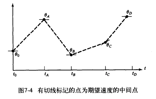
带有中间点的三次多项式轨迹规划,特点是中间点速度以及加速度连续
使用矩阵求解:
import numpy as np

def solve(theta0, thetav, thetag, tf1, tf2):
    """
    求解具有一个中间点的两段三次多项式系数
    """

    # A 矩阵: 8x8 系数矩阵 (对应 8 个未知系数 [a10, a11, a12, a13, a20, a21, a22, a23])
    # B 向量: 8x1 结果向量
    A = np.zeros((8, 8))
    B = np.zeros(8)

    # --- 第一段约束 (i=1) ---
    # 第一段起点位置
    A[0, 0] = 1
    B[0] = theta0

    # 第一段起点速度
    A[1, 1] = 1
    B[1] = 0

    # 第一段终点位置
    A[2, 0:4] = [1, tf1, tf1**2, tf1**3]
    B[2] = thetav

    # 第二段约束 (i=2) ---
    # 第二段起点位置
    A[3, 4] = 1
    B[3] = thetav

    # 第二段终点位置
    A[4, 4:8] = [1, tf2, tf2**2, tf2**3]
    B[4] = thetag

    # 第二段终点速度
    A[5, 5:8] = [1, 2*tf2, 3*tf2**2]
    B[5] = 0

    # 中间衔接约束
    A[6, 0:4] = [0, 1, 2*tf1, 3*tf1**2]
    A[6, 5] = -1
    B[6] = 0

    # 加速度连续
    A[7, 2:4] = [2, 6*tf1]
    A[7, 6] = -2
    B[7] = 0

    # 使用矩阵求逆或线性方程组求解器
    coeffs = np.linalg.solve(A, B)

    return coeffs

# 设定: 起点 0°, 中间点 45°, 终点 90°,每段耗时 1 秒
theta_start, theta_mid, theta_end = 0, 45, 90
t_f1, t_f2 = 1.0, 1.0

res = solve(theta_start, theta_mid, theta_end, t_f1, t_f2)

print("第一段系数 (a10, a11, a12, a13):", res[0:4])
print("第二段系数 (a20, a21, a22, a23):", res[4:8])

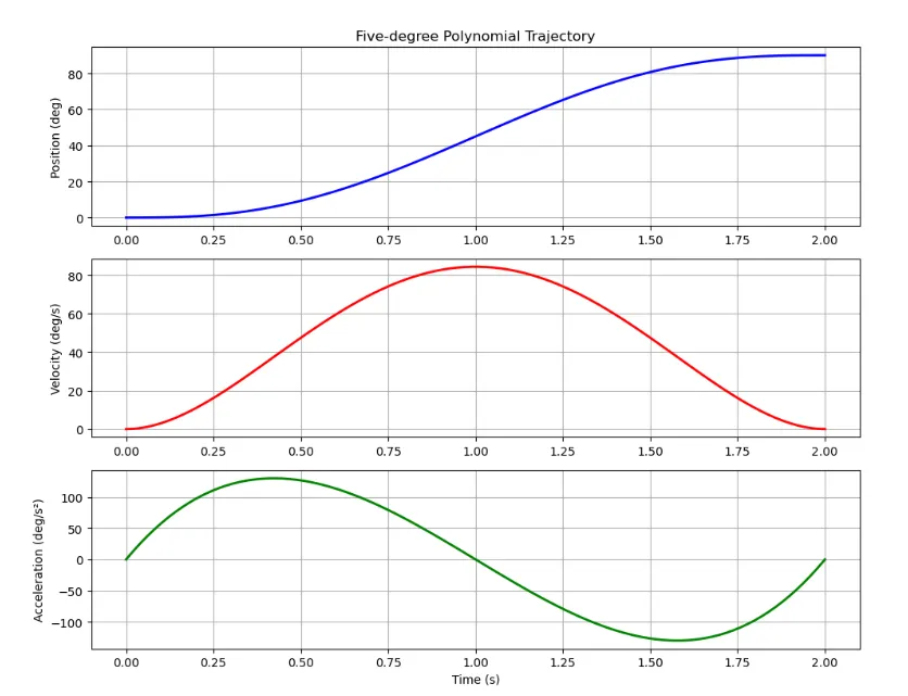
高阶多项式: 用五次多项式拟合,保证起点和终点的位置、速度、加速度连续。
有时用高阶多项式作为路径段。例如,如果要确定路径段起始点和终止点的位置、速度和加速度,则需要用一个五次多项式进行插值:
θ(t)=a0+a1t+a2t2+a3t3+a4t4+a5t5\theta(t) = a_0 + a_1 t + a_2 t^2 + a_3 t^3 + a_4 t^4 + a_5 t^5θ(t)=a0+a1t+a2t2+a3t3+a4t4+a5t5
其中,约束条件:
{θ0=a0θf=a0+a1tf+a2tf2+a3tf3+a4tf4+a5tf5θ˙0=a1θ˙f=a1+2a2tf+3a3tf2+4a4tf3+5a5tf4θ¨0=2a2θ¨f=2a2+6a3tf+12a4tf2+20a5tf3\begin{cases} \theta_0 = a_0 \\ \theta_f = a_0 + a_1 t_f + a_2 t_f^2 + a_3 t_f^3 + a_4 t_f^4 + a_5 t_f^5 \\ \dot{\theta}_0 = a_1 \\ \dot{\theta}_f = a_1 + 2a_2 t_f + 3a_3 t_f^2 + 4a_4 t_f^3 + 5a_5 t_f^4 \\ \ddot{\theta}_0 = 2a_2 \\ \ddot{\theta}_f = 2a_2 + 6a_3 t_f + 12a_4 t_f^2 + 20a_5 t_f^3 \end{cases}⎩
⎨
⎧θ0=a0θf=a0+a1tf+a2tf2+a3tf3+a4tf4+a5tf5θ˙0=a1θ˙f=a1+2a2tf+3a3tf2+4a4tf3+5a5tf4θ¨0=2a2θ¨f=2a2+6a3tf+12a4tf2+20a5tf3
这些约束条件确定了一个具有 6 个方程和 6 个未知数的线性方程组,其解为:
{a0=θ0a1=θ˙0a2=θ¨02a3=20θf−20θ0−(8θ˙f+12θ˙0)tf−(3θ¨0−θ¨f)tf22tf3a4=30θ0−30θf+(14θ˙f+16θ˙0)tf+(3θ¨0−2θ¨f)tf22tf4a5=12θf−12θ0−(6θ˙f+6θ˙0)tf−(θ¨0−θ¨f)tf22tf5\begin{cases} a_0 = \theta_0 \\ a_1 = \dot{\theta}_0 \\ a_2 = \dfrac{\ddot{\theta}_0}{2} \\ a_3 = \dfrac{20\theta_f - 20\theta_0 - (8\dot{\theta}_f + 12\dot{\theta}_0)t_f - (3\ddot{\theta}_0 - \ddot{\theta}_f)t_f^2}{2t_f^3} \\ a_4 = \dfrac{30\theta_0 - 30\theta_f + (14\dot{\theta}_f + 16\dot{\theta}_0)t_f + (3\ddot{\theta}_0 - 2\ddot{\theta}_f)t_f^2}{2t_f^4} \\ a_5 = \dfrac{12\theta_f - 12\theta_0 - (6\dot{\theta}_f + 6\dot{\theta}_0)t_f - (\ddot{\theta}_0 - \ddot{\theta}_f)t_f^2}{2t_f^5} \end{cases}⎩
⎨
⎧a0=θ0a1=θ˙0a2=2θ¨0a3=2tf320θf−20θ0−(8θ˙f+12θ˙0)tf−(3θ¨0−θ¨f)tf2a4=2tf430θ0−30θf+(14θ˙f+16θ˙0)tf+(3θ¨0−2θ¨f)tf2a5=2tf512θf−12θ0−(6θ˙f+6θ˙0)tf−(θ¨0−θ¨f)tf2
代码实现:
import numpy as np
import matplotlib.pyplot as plt

"""
    求解五次多项式系数
    参数: 起始/结束位置, 起始/结束速度, 起始/结束加速度, 总时长
"""

def solve_quintic_polynomial(theta0, thetaf, v0, vf, a0, af, tf):
    """_summary_

    Args:
        theta0 (_type_): 初始位置
        thetaf (_type_): 结束位置
        v0 (_type_): 初始速度
        vf (_type_): 结束速度
        a0 (_type_): 初始加速度
        af (_type_): 结束加速度
        tf (_type_): 总时长
    """
    # 构建6x6系数矩阵A
    # 方程组基于: theta(t), dot_theta(t), ddot_theta(t) 在 t=0 和 t=tf 的取值
    A = np.array([
        [1, 0,  0,   0,    0,     0],      # theta(0)
        [0, 1,  0,   0,    0,     0],      # dot_theta(0)
        [0, 0,  2,   0,    0,     0],      # ddot_theta(0)
        [1, tf, tf**2, tf**3, tf**4, tf**5], # theta(tf)
        [0, 1,  2*tf, 3*tf**2, 4*tf**3, 5*tf**4], # dot_theta(tf)
        [0, 0,  2,   6*tf, 12*tf**2, 20*tf**3]  # ddot_theta(tf)
    ])

    # 构建6x1结果向量B
    B = np.array([theta0, v0, a0, thetaf, vf, af])

    # 求解线性方程组 Ax = B
    # coeffs 包含 [a0, a1, a2, a3, a4, a5]
    coeffs = np.linalg.solve(A, B)
    return coeffs

# 从 0° 运动到 90°,用时 2 秒
# 起始和结束的速度、加速度均为 0
t_final = 2.0
a_coeffs = solve_quintic_polynomial(0, 90, 0, 0, 0, 0, t_final)

# 生成轨迹数据进行绘图
t = np.linspace(0, t_final, 100)
pos = a_coeffs[0] + a_coeffs[1]*t + a_coeffs[2]*t**2 + a_coeffs[3]*t**3 + a_coeffs[4]*t**4 + a_coeffs[5]*t**5 # 位置
vel = a_coeffs[1] + 2*a_coeffs[2]*t + 3*a_coeffs[3]*t**2 + 4*a_coeffs[4]*t**3 + 5*a_coeffs[5]*t**4 # 速度
acc = 2*a_coeffs[2] + 6*a_coeffs[3]*t + 12*a_coeffs[4]*t**2 + 20*a_coeffs[5]*t**3 # 加速度

print("五次多项式系数:", a_coeffs)

plt.figure(figsize=(10, 8))

# 1:位置曲线
plt.subplot(3, 1, 1)
plt.plot(t, pos, 'b', linewidth=2)
plt.title('Five-degree Polynomial Trajectory')
plt.ylabel('Position (deg)')
plt.grid(True)

# 2:速度曲线
plt.subplot(3, 1, 2)
plt.plot(t, vel, 'r', linewidth=2)
plt.ylabel('Velocity (deg/s)')
plt.grid(True)

# 3:加速度曲线
plt.subplot(3, 1, 3)
plt.plot(t, acc, 'g', linewidth=2)
plt.ylabel('Acceleration (deg/s²)')
plt.xlabel('Time (s)')
plt.grid(True)

plt.tight_layout()
plt.show()

笛卡尔空间规划方法
| 特性 | 基于欧拉角姿态规划 | 基于等效轴角姿态规划 |
|---|---|---|
| 姿态表示 | 3个欧拉角(有依赖) | 1个轴+1个角度(无依赖) |
| 插值逻辑 | 对3个角度分别插值 | 对1个角度插值(轴固定) |
| 万向锁风险 | 存在(严重缺陷) | 无(核心优势) |
| 平滑性 | 可能突变 | 连续稳定 |
| 适用场景 | 低精度、简单运动 | 高精度、高稳定性运动 |
基本规划算法
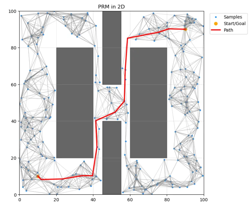
概率路图算法(Probabilistic Road Map, PRM)
import numpy as np
import matplotlib.pyplot as plt
import heapq
import random

# --- 环境设置 ---
bounds = (0, 100, 0, 100)  # xmin, xmax, ymin, ymax
obstacles = [
    (20, 40, 20, 80),
    (60, 80, 20, 80),
    (45, 55, 0, 40),
    (45, 55, 60, 100)
]
start = np.array([10, 10])
goal = np.array([90, 90])
clearance = 0.8  # 与障碍的安全间隙

# --- 碰撞检测 ---
def rect_with_margin(rect, m):
    xmin, xmax, ymin, ymax = rect
    return (xmin - m, xmax + m, ymin - m, ymax + m)

def in_obstacle(p):
    p = np.asarray(p, dtype=float).reshape(2, -1)
    x = p[0]
    y = p[1]
    for rect in obstacles:
        xmin, xmax, ymin, ymax = rect_with_margin(rect, clearance)
        inside = (xmin <= x) & (x <= xmax) & (ymin <= y) & (y <= ymax)
        if np.any(inside):
            return True
    return False

def orient(a, b, c):
    return (b[0] - a[0]) * (c[1] - a[1]) - (b[1] - a[1]) * (c[0] - a[0])

def on_segment(a, b, c, eps=1e-9):
    return (min(a[0], b[0]) - eps <= c[0] <= max(a[0], b[0]) + eps and
            min(a[1], b[1]) - eps <= c[1] <= max(a[1], b[1]) + eps)

def segments_intersect(a, b, c, d):
    o1 = orient(a, b, c)
    o2 = orient(a, b, d)
    o3 = orient(c, d, a)
    o4 = orient(c, d, b)
    eps = 1e-9
    if (o1 > eps and o2 < -eps) or (o1 < -eps and o2 > eps):
        if (o3 > eps and o4 < -eps) or (o3 < -eps and o4 > eps):
            return True
    if abs(o1) <= eps and on_segment(a, b, c):
        return True
    if abs(o2) <= eps and on_segment(a, b, d):
        return True
    if abs(o3) <= eps and on_segment(c, d, a):
        return True
    if abs(o4) <= eps and on_segment(c, d, b):
        return True
    return False

def segment_intersects_rect(p1, p2, rect):
    xmin, xmax, ymin, ymax = rect_with_margin(rect, clearance)
    # 端点在矩形内
    if xmin <= p1[0] <= xmax and ymin <= p1[1] <= ymax:
        return True
    if xmin <= p2[0] <= xmax and ymin <= p2[1] <= ymax:
        return True
    # 与四条边相交
    corners = [(xmin, ymin), (xmax, ymin), (xmax, ymax), (xmin, ymax)]
    edges = [
        (corners[0], corners[1]),
        (corners[1], corners[2]),
        (corners[2], corners[3]),
        (corners[3], corners[0])
    ]
    for c, d in edges:
        if segments_intersect(p1, p2, c, d):
            return True
    return False

def segment_free(p1, p2):
    if in_obstacle(p1) or in_obstacle(p2):
        return False
    for rect in obstacles:
        if segment_intersects_rect(p1, p2, rect):
            return False
    return True

# --- 采样 ---
def sample_free(n):
    pts = []
    xmin, xmax, ymin, ymax = bounds
    while len(pts) < n:
        x = random.uniform(xmin, xmax)
        y = random.uniform(ymin, ymax)
        p = np.array([x, y])
        if not in_obstacle(p):
            pts.append(p)
    return np.array(pts)

# --- 构建路标图 ---
def build_roadmap(points, k=10):
    n = len(points)
    edges = [[] for _ in range(n)]
    for i in range(n):
        dists = np.linalg.norm(points - points[i], axis=1)
        idx = np.argsort(dists)
        for j in idx[1:k+1]:
            if segment_free(points[i], points[j]):
                w = dists[j]
                edges[i].append((j, w))
                edges[j].append((i, w))
    return edges

# --- Dijkstra ---
def dijkstra(edges, s, g):
    n = len(edges)
    dist = [float('inf')] * n
    prev = [-1] * n
    dist[s] = 0.0
    pq = [(0.0, s)]
    while pq:
        d, u = heapq.heappop(pq)
        if u == g:
            break
        if d != dist[u]:
            continue
        for v, w in edges[u]:
            nd = d + w
            if nd < dist[v]:
                dist[v] = nd
                prev[v] = u
                heapq.heappush(pq, (nd, v))
    if dist[g] == float('inf'):
        return None
    path = []
    cur = g
    while cur != -1:
        path.append(cur)
        cur = prev[cur]
    return path[::-1]

# --- 运行 PRM ---
np.random.seed(0)
random.seed(0)
samples = sample_free(250)
points = np.vstack([start, goal, samples])
edges = build_roadmap(points, k=12)
path_idx = dijkstra(edges, 0, 1)

# --- 绘图 ---
plt.figure(figsize=(7.5, 7))
for (xmin, xmax, ymin, ymax) in obstacles:
    plt.fill([xmin, xmax, xmax, xmin], [ymin, ymin, ymax, ymax], color='black', alpha=0.6)
plt.scatter(points[2:, 0], points[2:, 1], s=8, c='dodgerblue', label='Samples')
plt.scatter([start[0], goal[0]], [start[1], goal[1]], c='orange', s=50, label='Start/Goal')
for i, nbrs in enumerate(edges):
    for j, _ in nbrs:
        if j > i:
            plt.plot([points[i, 0], points[j, 0]], [points[i, 1], points[j, 1]], color='gray', linewidth=0.5, alpha=0.5)
if path_idx is not None:
    path = points[path_idx]
    plt.plot(path[:, 0], path[:, 1], color='red', linewidth=2.5, label='Path')
plt.xlim(bounds[0], bounds[1])
plt.ylim(bounds[2], bounds[3])
plt.gca().set_aspect('equal', adjustable='box')
plt.title('PRM in 2D')
plt.legend(loc='upper left', bbox_to_anchor=(1.02, 1.0), frameon=True)
plt.grid(True, alpha=0.3)
plt.tight_layout()
plt.show()
快速随机扩展树算法(Rapidly-exploring Random Tree, RRT)
RRT 是一种增量式在线规划算法,核心是通过随机采样不断扩展一棵 “搜索树”,最终连接起点和终点,适合动态、未知环境的在线路径规划。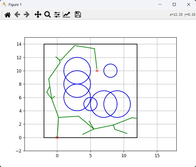
问题:
轨迹规划时,为什么要限制速度和加速度?
比如电机控制关节的机械臂来说,电机存在最大转速,要控制速度及加速度;保证机械臂稳定性在可控范围内;保证控制安全等等。
如果规定两秒钟必须完成一次动作,应该如何安排轨迹?
可采用梯形速度曲线控制算法。梯形速度曲线将整个运动过程分为匀加速、匀速和匀减速三个阶段,在变速过程中加速度保持不变。

DAMO开发者矩阵,由阿里巴巴达摩院和中国互联网协会联合发起,致力于探讨最前沿的技术趋势与应用成果,搭建高质量的交流与分享平台,推动技术创新与产业应用链接,围绕“人工智能与新型计算”构建开放共享的开发者生态。
更多推荐


 13
13 0
0- 0


 已为社区贡献3条内容

所有评论(0)