SLAM文献之A micro Lie theory for state estimation in robotic(4)
相关内容地址:1、SLAM文献之A micro Lie theory for state estimation in robotic(1)2、SLAM文献之A micro Lie theory for state estimation in robotic(2)3、SLAM文献之A micro Lie theory for state estimation in robotic(3)我们以一种适合
相关内容地址:
1、SLAM文献之A micro Lie theory for state estimation in robotic(1)
2、SLAM文献之A micro Lie theory for state estimation in robotic(2)
3、SLAM文献之A micro Lie theory for state estimation in robotic(3)
VI. 结论
我们以一种适合具备状态估计背景读者的形式,介绍了李群理论的核心内容,并重点关注机器人学的应用。我们通过以下几个方面来实现这一目标:
首先,选择了尽可能避免抽象数学概念的材料。这有助于聚焦李群理论,使其工具更易于理解和使用。
其次,采用了教学性的方法,内容具有显著冗余性。正文内容是通用的,涵盖了李群理论的抽象要点。同时配有方框示例,将抽象概念具体化到特定李群,并提供大量配有详细说明的图示。
第三,我们推广了方便使用的算子,例如大写的 E x p ( ) Exp() Exp() 和 L o g ( ) Log() Log() 映射,以及加减算子 ⊕ , ⊖ \oplus, \ominus ⊕,⊖ 等。它们允许我们在切空间的笛卡尔表示下工作,从而得到的导数和协方差处理公式与标准向量空间中的对应公式高度相似。
第四,我们特别强调了雅可比矩阵的定义、几何解释及计算方法。为此,我们引入了雅可比矩阵和协方差的符号,使得操作直观且易于理解。尤其是链式法则在此符号体系下非常清晰,有助于建立直觉并减少错误。
第五,附录中提供了机器人学中最常用李群的公式大全。在二维中,我们展示了单位复数旋转群 S 1 S^1 S1、旋转矩阵群 S O ( 2 ) SO(2) SO(2) 以及刚体运动群 S E ( 2 ) SE(2) SE(2);在三维中,我们展示了单位四元数群 S 3 S^3 S3、旋转矩阵群 S O ( 3 ) SO(3) SO(3) 以及刚体运动群 S E ( 3 ) SE(3) SE(3)。同时,我们还提供了任意维度的平移群,可通过标准向量空间 R n \mathbb{R}^n Rn 的加法或矩阵平移群 T ( n ) T(n) T(n) 的乘法来实现。
第六,我们给出了一些应用示例,展示了李群理论在机器人问题中以优雅且精确的方式求解问题的能力。复合群的概念虽略显朴素,但有助于将异构状态向量统一为李群理论形式。
最后,我们附带了新的 C++ 库 manif [7],实现了本文描述的工具。manif 可在 https://github.com/artivis/manif 获取。第 V 节中的应用示例也在 manif 中得到了演示。
尽管本文并未引入新的理论内容,但我们相信,本文呈现李群理论的形式将帮助许多研究人员进入该领域,为其未来研究提供便利。我们也认为,这本身就是一项有价值的贡献。
附录 A
二维旋转群 S 1 S^1 S1 与 S O ( 2 ) SO(2) SO(2)
李群 S 1 S^1 S1 是单位复数在复数乘法下的群。其拓扑是单位圆或单位 1-球,因此得名 S 1 S^1 S1。该群、李代数和向量元素形式为:
z = cos θ + i sin θ , τ ∧ = i θ , τ = θ . (112) z = \cos\theta + i \sin\theta, \quad \tau^\wedge = i \theta, \quad \tau = \theta. \tag{112} z=cosθ+isinθ,τ∧=iθ,τ=θ.(112)
取逆和复合通过共轭实现: z − 1 = z ∗ z^{-1} = z^* z−1=z∗,复合为 z a ∘ z b = z a z b z_a \circ z_b = z_a z_b za∘zb=zazb。
群 S O ( 2 ) SO(2) SO(2) 是平面内特殊正交矩阵群,即旋转矩阵群,在矩阵乘法下构成群。群、李代数和向量元素形式为:
R = [ cos θ − sin θ sin θ cos θ ] , τ ∧ = [ θ ] × = [ 0 − θ θ 0 ] , τ = θ . (113) R = \begin{bmatrix} \cos\theta & -\sin\theta \\ \sin\theta & \cos\theta \end{bmatrix}, \quad \tau^\wedge = [\theta]_\times = \begin{bmatrix} 0 & -\theta \\ \theta & 0 \end{bmatrix}, \quad \tau = \theta. \tag{113} R=[cosθsinθ−sinθcosθ],τ∧=[θ]×=[0θ−θ0],τ=θ.(113)
取逆和复合通过转置实现: R − 1 = R ⊤ R^{-1} = R^\top R−1=R⊤,复合为 R a ∘ R b = R a R b R_a \circ R_b = R_a R_b Ra∘Rb=RaRb。
两者都作用于二维向量,并且切空间同构,因此可以一起研究。
A. Exp 与 Log 映射
S 1 S^1 S1 和 S O ( 2 ) SO(2) SO(2) 的复数与旋转矩阵可以定义 Exp 与 Log 映射。
对于 S 1 S^1 S1:
z = Exp ( θ ) = cos θ + i sin θ ∈ C , (114) z = \text{Exp}(\theta) = \cos\theta + i \sin\theta \in \mathbb{C}, \tag{114} z=Exp(θ)=cosθ+isinθ∈C,(114)
θ = Log ( z ) = arctan ( Im ( z ) , Re ( z ) ) ∈ R , (115) \theta = \text{Log}(z) = \arctan(\text{Im}(z), \text{Re}(z)) \in \mathbb{R}, \tag{115} θ=Log(z)=arctan(Im(z),Re(z))∈R,(115)
其中 (114) 为欧拉公式。
对于 S O ( 2 ) SO(2) SO(2):
R = Exp ( θ ) = [ cos θ − sin θ sin θ cos θ ] ∈ R 2 × 2 , (116) R = \text{Exp}(\theta) = \begin{bmatrix} \cos\theta & -\sin\theta \\ \sin\theta & \cos\theta \end{bmatrix} \in \mathbb{R}^{2 \times 2}, \tag{116} R=Exp(θ)=[cosθsinθ−sinθcosθ]∈R2×2,(116)
θ = Log ( R ) = arctan ( r 21 , r 11 ) ∈ R . (117) \theta = \text{Log}(R) = \arctan(r_{21}, r_{11}) \in \mathbb{R}. \tag{117} θ=Log(R)=arctan(r21,r11)∈R.(117)
B. 取逆、复合与指数映射
考虑通用二维旋转元素,用无衬线字体表示 Q , R Q, R Q,R:
R ( θ ) − 1 = R ( − θ ) , (118) R(\theta)^{-1} = R(-\theta), \tag{118} R(θ)−1=R(−θ),(118)
Q ∘ R = R ∘ Q , (119) Q \circ R = R \circ Q, \tag{119} Q∘R=R∘Q,(119)
即平面旋转是可交换的。因此有:
Exp ( θ 1 + θ 2 ) = Exp ( θ 1 ) ∘ Exp ( θ 2 ) , (120) \text{Exp}(\theta_1 + \theta_2) = \text{Exp}(\theta_1) \circ \text{Exp}(\theta_2), \tag{120} Exp(θ1+θ2)=Exp(θ1)∘Exp(θ2),(120)
Log ( Q ∘ R ) = Log ( Q ) + Log ( R ) , (121) \text{Log}(Q \circ R) = \text{Log}(Q) + \text{Log}(R), \tag{121} Log(Q∘R)=Log(Q)+Log(R),(121)
Q ⊖ R = θ Q − θ R . (122) Q \ominus R = \theta_Q - \theta_R. \tag{122} Q⊖R=θQ−θR.(122)
C. 雅可比块
由于我们定义的导数映射切向量空间,并且对于 S 1 S^1 S1 和 S O ( 2 ) SO(2) SO(2) 的平面旋转流形,这些空间相同,即 θ = Log ( z ) = Log ( R ) \theta = \text{Log}(z) = \text{Log}(R) θ=Log(z)=Log(R),所以雅可比与表示方式( z z z 或 R R R)无关。
1) 伴随与其他平凡雅可比:
由 (41a)、第 III-B 节及以上性质,有以下标量导数块为平凡值:
Ad R = 1 ∈ R , (123) \text{Ad}_R = 1 \in \mathbb{R}, \tag{123} AdR=1∈R,(123)
J R − 1 R = − 1 ∈ R , (124) J_{R^{-1}}^R = -1 \in \mathbb{R}, \tag{124} JR−1R=−1∈R,(124)
J Q Q ∘ R = J Q R ∘ R = 1 ∈ R , (125) J_{Q}^{Q \circ R} = J_Q^{R \circ R} = 1 \in \mathbb{R}, \tag{125} JQQ∘R=JQR∘R=1∈R,(125)
J r ( θ ) = J l ( θ ) = 1 ∈ R , (126) J_r(\theta) = J_l(\theta) = 1 \in \mathbb{R}, \tag{126} Jr(θ)=Jl(θ)=1∈R,(126)
J R R ⊕ θ = J R θ ⊕ θ = 1 ∈ R , (127) J_R^{R \oplus \theta} = J_R^{\theta \oplus \theta} = 1 \in \mathbb{R}, \tag{127} JRR⊕θ=JRθ⊕θ=1∈R,(127)
J Q Q ⊖ R = − J R Q ⊖ R = 1 ∈ R . (128) J_Q^{Q \ominus R} = -J_R^{Q \ominus R} = 1 \in \mathbb{R}. \tag{128} JQQ⊖R=−JRQ⊖R=1∈R.(128)
2) 旋转作用
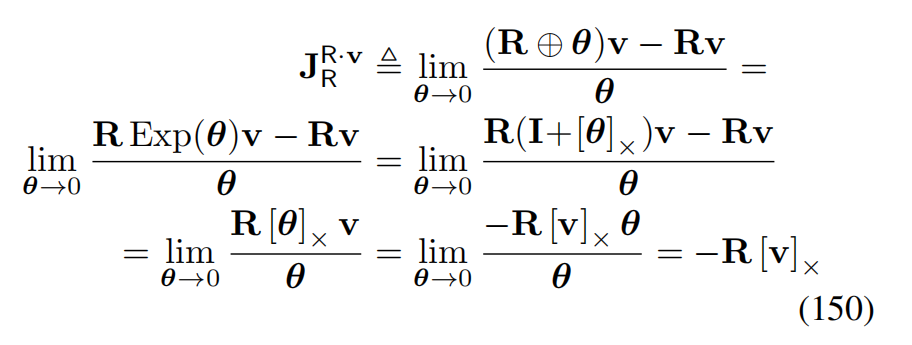
对于作用 R ⋅ v R \cdot v R⋅v:
J R R ⋅ v = lim θ → 0 R Exp ( θ ) v − R v θ = lim θ → 0 R ( I + [ θ ] × ) v − R v θ = lim θ → 0 R [ θ ] × v θ = R [ 1 ] × v ∈ R 2 × 1 , (129) J_R^{R \cdot v} = \lim_{\theta \to 0} \frac{R \text{Exp}(\theta) v - Rv}{\theta}\\ = \lim_{\theta \to 0} \frac{R(I + [\theta]\times)v - Rv}{\theta}\\ = \lim{\theta \to 0} \frac{R[\theta]\times v}{\theta}\\ = R[1]\times v \in \mathbb{R}^{2 \times 1}, \tag{129} JRR⋅v=θ→0limθRExp(θ)v−Rv=θ→0limθR(I+[θ]×)v−Rv=limθ→0θR[θ]×v=R[1]×v∈R2×1,(129)
J v R v ⋅ = D ( R v ) D v = R ∈ R 2 × 2 . (130) J^{Rv \cdot }_v = \frac{D(Rv)}{Dv} = R \in \mathbb{R}^{2 \times 2}. \tag{130} JvRv⋅=DvD(Rv)=R∈R2×2.(130)
附录 B
三维旋转群 S 3 S^3 S3 与 S O ( 3 ) SO(3) SO(3)
李群 S 3 S^3 S3 是单位四元数在四元数乘法下的群。其拓扑是 R 4 \mathbb{R}^4 R4 中的单位 3-球,因此得名 S 3 S^3 S3。四元数(详见参考文献 [8])可以用以下等价形式表示:
q = w + i x + j y + k z = w + v ∈ H = [ w x y z ] ⊤ = [ w v ] ∈ H , (131) q = w + ix + jy + kz = w + \mathbf{v} \in \mathbb{H}\\ = \begin{bmatrix} w & x & y & z \end{bmatrix}^\top = \begin{bmatrix} w \\ \mathbf{v} \end{bmatrix} \in \mathbb{H}, \tag{131} q=w+ix+jy+kz=w+v∈H=[wxyz]⊤=[wv]∈H,(131)
其中 w , x , y , z ∈ R w, x, y, z \in \mathbb{R} w,x,y,z∈R, i , j , k i,j,k i,j,k 为三个单位虚数,满足 i 2 = j 2 = k 2 = i j k = − 1 i^2 = j^2 = k^2 = ijk = -1 i2=j2=k2=ijk=−1。标量 w w w 为实部, v ∈ H p \mathbf{v} \in \mathbb{H}_p v∈Hp 为向量部(纯虚部),维度为 3。取逆与复合通过共轭实现 q − 1 = q ∗ q^{-1} = q^* q−1=q∗,其中 q ∗ = w − v q^* = w - \mathbf{v} q∗=w−v,复合为 q a ∘ q b = q a q b q_a \circ q_b = q_a q_b qa∘qb=qaqb。
群 S O ( 3 ) SO(3) SO(3) 是三维空间中的特殊正交矩阵群,即旋转矩阵群,在矩阵乘法下构成群。取逆与复合通过转置和矩阵乘法实现,与 S O ( n ) SO(n) SO(n) 类似。
两者都作用于三维向量,其切空间同构,可用 R 3 \mathbb{R}^3 R3 的旋转向量表示,因此可一起研究。在此空间中,我们定义旋转速度向量 ω ≜ u ω \omega \triangleq u\omega ω≜uω,轴角 θ ≜ u θ \theta \triangleq u\theta θ≜uθ 以及所有扰动和不确定性。
四元数流形 S 3 S^3 S3 是 S O ( 3 ) SO(3) SO(3) 的双覆盖,即 q q q 和 − q -q −q 表示同一旋转 R R R。第一覆盖对应实部 w > 0 w>0 w>0 的四元数。两群在第一覆盖下可视为同构。
A. Exp 与 Log 映射
四元数 q = ( w , v ) ∈ H q=(w,\mathbf{v}) \in \mathbb{H} q=(w,v)∈H 的 Exp 与 Log 映射(参见例 5):
q = Exp ( θ u ) ≜ cos ( θ / 2 ) + u sin ( θ / 2 ) ∈ H , (132) q = \text{Exp}(\theta \mathbf{u}) \triangleq \cos(\theta/2) + \mathbf{u} \sin(\theta/2) \in \mathbb{H}, \tag{132} q=Exp(θu)≜cos(θ/2)+usin(θ/2)∈H,(132)
θ u = Log ( q ) ≜ 2 v ∣ ∣ v ∣ ∣ arctan ( ∣ ∣ v ∣ ∣ , w ) ∈ R 3 . (133) \theta \mathbf{u} = \text{Log}(q) \triangleq 2 \frac{\mathbf{v}}{||\mathbf{v}||} \arctan\ (||\mathbf{v}||{,w}) \in \mathbb{R}^3. \tag{133} θu=Log(q)≜2∣∣v∣∣varctan (∣∣v∣∣,w)∈R3.(133)
为避免双覆盖问题,可确保实部 w > 0 w>0 w>0,若不满足,可用 − q -q −q 替换 q q q。
旋转矩阵的 Exp 与 Log(参见例 4):
R = Exp ( θ u ) ≜ I + sin θ [ u ] × + ( 1 − cos θ ) [ u ] × 2 ∈ R 3 × 3 , (134) R = \text{Exp}(\theta \mathbf{u}) \triangleq I + \sin\theta [\mathbf{u}]\times + (1-\cos\theta) [\mathbf{u}]\times^2 \in \mathbb{R}^{3\times 3}, \tag{134} R=Exp(θu)≜I+sinθ[u]×+(1−cosθ)[u]×2∈R3×3,(134)
θ u = Log ( R ) ≜ θ ( R − R ⊤ ) ∨ 2 sin θ ∈ R 3 , (135) \theta \mathbf{u} = \text{Log}(R) \triangleq \frac{\theta(R-R^\top)^\vee}{2 \sin\theta} \in \mathbb{R}^3, \tag{135} θu=Log(R)≜2sinθθ(R−R⊤)∨∈R3,(135)
其中 θ = cos − 1 ( trace ( R ) − 1 2 ) \theta = \cos^{-1}\left(\frac{\text{trace}(R)-1}{2}\right) θ=cos−1(2trace(R)−1)。
B. 旋转作用
四元数对三维向量的旋转作用通过双四元数乘法实现:
x ′ = q x q ∗ , (136) \mathbf{x}' = q \mathbf{x} q^*, \tag{136} x′=qxq∗,(136)
旋转矩阵通过单矩阵乘法实现:
x ′ = R x . (137) \mathbf{x}' = R \mathbf{x}. \tag{137} x′=Rx.(137)
两者均对应绕轴 u \mathbf{u} u 顺时针旋转 θ \theta θ 弧度。由此可得到 q q q 对应的旋转矩阵:
R ( q ) = [ w 2 + x 2 − y 2 − z 2 2 ( x y − w z ) 2 ( x z + w y ) 2 ( x y + w z ) w 2 − x 2 + y 2 − z 2 2 ( y z − w x ) 2 ( x z − w y ) 2 ( y z + w x ) w 2 − x 2 − y 2 + z 2 ] . (138) R(q) = \begin{bmatrix} w^2+x^2-y^2-z^2 & 2(xy-wz) & 2(xz+wy) \\ 2(xy+wz) & w^2-x^2+y^2-z^2 & 2(yz-wx) \\ 2(xz-wy) & 2(yz+wx) & w^2-x^2-y^2+z^2 \end{bmatrix}. \tag{138} R(q)= w2+x2−y2−z22(xy+wz)2(xz−wy)2(xy−wz)w2−x2+y2−z22(yz+wx)2(xz+wy)2(yz−wx)w2−x2−y2+z2 .(138)
C. 基本雅可比块
由于定义的导数映射切向量空间,对于 S 3 S^3 S3 和 S O ( 3 ) SO(3) SO(3) 的 3D 旋转流形, θ = Log ( q ) = Log ( R ) \theta = \text{Log}(q) = \text{Log}(R) θ=Log(q)=Log(R),雅可比与表示方式无关( q q q或 R R R)。
考虑通用 3D 旋转元素,记为 R R R:
1) 伴随
由 (31) 得:
Ad R θ = ( R [ θ ] × R ⊤ ) ∨ = ( [ R θ ] × ) ∨ = R θ ⟹ Ad R = R . (139) \text{Ad}_R \theta = (R [\theta]\times R^\top)^\vee = ([R\theta]_\times)^\vee = R \theta \implies \\ \text{Ad}_R = R. \tag{139} AdRθ=(R[θ]×R⊤)∨=([Rθ]×)∨=Rθ⟹AdR=R.(139)
说明 Ad q = R ( q ) \text{Ad}_q = R(q) Adq=R(q)(见 (138)), Ad R = R \text{Ad}_R = R AdR=R。
2) 取逆与复合
由 III-B 节得:
J R − 1 R = − Ad R = − R , (140) J_{R^{-1}}^R = -\text{Ad}_R = -R, \tag{140} JR−1R=−AdR=−R,(140)
J Q Q R = Ad R − 1 = R ⊤ , (141) J^{QR}_Q = \text{Ad}_{R}^{-1} = R^\top, \tag{141} JQQR=AdR−1=R⊤,(141)
J R Q R = I . (142) J^{QR}_R = I. \tag{142} JRQR=I.(142)
3) 左右雅可比
闭式形式([11, 页 40]):
J r ( θ ) = I − 1 − cos θ θ 2 [ θ ] × + θ − sin θ θ 3 [ θ ] 2 × , (143) J_r(\theta) = I - \frac{1-\cos\theta}{\theta^2} [\theta]\times + \frac{\theta-\sin\theta}{\theta^3} [\theta]^2\times, \tag{143} Jr(θ)=I−θ21−cosθ[θ]×+θ3θ−sinθ[θ]2×,(143)
J r − 1 ( θ ) = I + 1 2 [ θ ] × + ( θ 2 − 1 + cos θ 2 θ sin θ ) [ θ ] 2 × , (144) J_r^{-1}(\theta) = I + \frac{1}{2}[\theta]\times + \left(\frac{\theta}{2} - \frac{1+\cos\theta}{2\theta \sin\theta}\right)[\theta]^2\times, \tag{144} Jr−1(θ)=I+21[θ]×+(2θ−2θsinθ1+cosθ)[θ]2×,(144)
J l ( θ ) = I + 1 − cos θ θ 2 [ θ ] × + θ − sin θ θ 3 [ θ ] 2 × , (145) J_l(\theta) = I + \frac{1-\cos\theta}{\theta^2} [\theta]\times + \frac{\theta-\sin\theta}{\theta^3} [\theta]^2\times, \tag{145} Jl(θ)=I+θ21−cosθ[θ]×+θ3θ−sinθ[θ]2×,(145)
J l − 1 ( θ ) = I − 1 2 [ θ ] × + ( θ 2 − 1 + cos θ 2 θ sin θ ) [ θ ] 2 × . (146) J_l^{-1}(\theta) = I - \frac{1}{2}[\theta]\times + \left(\frac{\theta}{2} - \frac{1+\cos\theta}{2\theta \sin\theta}\right)[\theta]^2\times. \tag{146} Jl−1(θ)=I−21[θ]×+(2θ−2θsinθ1+cosθ)[θ]2×.(146)
可观察到:
J l = J r ⊤ , J l − 1 = J r − ⊤ . (147) J_l = J_r^\top, \quad J_l^{-1} = J_r^{- \top}. \tag{147} Jl=Jr⊤,Jl−1=Jr−⊤.(147)
4) 右加与右减
对于 θ = Q ⊖ R \theta = Q \ominus R θ=Q⊖R:
J R R ⊕ θ = R ( θ ) ⊤ , J R θ ⊕ θ = J r ( θ ) , (148) J_R^{R \oplus \theta} = R(\theta)^\top, \quad J_R^{\theta \oplus \theta} = J_r(\theta), \tag{148} JRR⊕θ=R(θ)⊤,JRθ⊕θ=Jr(θ),(148)
J Q Q ⊖ R = J r 1 − ( θ ) , J R Q ⊖ R = − J l 1 − ( θ ) . (149) J_Q^{Q \ominus R} = J_{r1}^-(\theta), \quad J_R^{Q \ominus R} = -J_{l1}^-(\theta). \tag{149} JQQ⊖R=Jr1−(θ),JRQ⊖R=−Jl1−(θ).(149)
5) 旋转作用
利用了 Exp ( θ ) ≈ I + [ θ ] × \text{Exp}(\theta) \approx I + [\theta]\times Exp(θ)≈I+[θ]× 与 [ a ] × b = − [ b ] × a [a]\times b = -[b]_\times a [a]×b=−[b]×a。
第二个雅可比为:
J v R ⋅ v = lim Δ v → 0 R ( v + Δ v ) − R v Δ v = R . (151) J^{R \cdot v}_v = \lim_{\Delta v \to 0} \frac{R(v+\Delta v)-Rv}{\Delta v} = R. \tag{151} JvR⋅v=Δv→0limΔvR(v+Δv)−Rv=R.(151)
附录 C
二维刚体运动群 S E ( 2 ) SE(2) SE(2)
我们将刚体运动群 S E ( 2 ) SE(2) SE(2) 的元素表示为
M = [ R t 0 1 ] ∈ S E ( 2 ) ⊂ R 3 × 3 , (152) M = \begin{bmatrix} R & t \\ 0 & 1 \end{bmatrix} \in SE(2) \subset \mathbb{R}^{3 \times 3}, \tag{152} M=[R0t1]∈SE(2)⊂R3×3,(152)
其中 R ∈ S O ( 2 ) R \in SO(2) R∈SO(2) 为旋转, t ∈ R 2 t \in \mathbb{R}^2 t∈R2 为平移。李代数和向量切空间由如下元素构成:
τ ∧ = [ [ θ ] × ρ 0 0 ] ∈ s e ( 2 ) , τ = [ ρ θ ] ∈ R 3 . (153) \tau^\wedge = \begin{bmatrix} [\theta]_ \times & \rho \\ 0 & 0 \end{bmatrix} \in se(2), \quad \tau = \begin{bmatrix} \rho \\ \theta \end{bmatrix} \in \mathbb{R}^3. \tag{153} τ∧=[[θ]×0ρ0]∈se(2),τ=[ρθ]∈R3.(153)
A. 取逆与复合
取逆与复合分别通过矩阵求逆与矩阵乘法实现:
M − 1 = [ R ⊤ − R ⊤ t 0 1 ] , (154) M^{-1} = \begin{bmatrix} R^\top & -R^\top t \\ 0 & 1 \end{bmatrix}, \tag{154} M−1=[R⊤0−R⊤t1],(154)
M a M b = [ R a R b t a + t b 0 1 ] . (155) M_a M_b = \begin{bmatrix} R_a & R_b t_a + t_b \\ 0 \ & 1 \end{bmatrix}. \tag{155} MaMb=[Ra0 Rbta+tb1].(155)
B. Exp 与 Log 映射
Exp 与 Log 通过标量切空间 R 3 ≃ s e ( 2 ) = T S E ( 2 ) \mathbb{R}^3 \simeq se(2) = TSE(2) R3≃se(2)=TSE(2) 的指数映射实现(参见 [5]):
M = Exp ( τ ) ≜ [ Exp ( [ 0 θ ] ) V 1 ( θ ) ρ 0 1 ] , (156) M = \text{Exp}(\tau) \triangleq \begin{bmatrix} \text{Exp}([0\ \theta]) & V_1(\theta) \rho \\ 0 & 1 \end{bmatrix}, \tag{156} M=Exp(τ)≜[Exp([0 θ])0V1(θ)ρ1],(156)
τ = Log ( M ) ≜ [ V − 1 ( θ ) t Log ( R ) ] , (157) \tau = \text{Log}(M) \triangleq \begin{bmatrix} V^{-1}(\theta) t \\ \text{Log}(R) \end{bmatrix}, \tag{157} τ=Log(M)≜[V−1(θ)tLog(R)],(157)
其中
V ( θ ) = sin θ θ I + 1 − cos θ θ [ 1 ] × . (158) V(\theta) = \frac{\sin \theta}{\theta} I + \frac{1-\cos\theta}{\theta} [1]_\times. \tag{158} V(θ)=θsinθI+θ1−cosθ[1]×.(158)
C. 雅可比块
1) 伴随
由 (31) 并利用平面旋转可交换性,可得:
Ad M τ = ( M τ ∧ M − 1 ) ∨ = [ R ρ − θ [ 1 ] × t θ ] = Ad M [ ρ θ ] , Ad M = [ R − [ 1 ] × t 0 1 ] . (159) \text{Ad}_M \tau = (M \tau^\wedge M^{-1})^\vee = \begin{bmatrix} R \rho - \theta [1]\times t \\ \theta \end{bmatrix} = \text{Ad}_M \begin{bmatrix} \rho \\ \theta \end{bmatrix},\\ \quad \text{Ad}_M = \begin{bmatrix} R & -[1]\times t \\0 \ & 1 \end{bmatrix}. \tag{159} AdMτ=(Mτ∧M−1)∨=[Rρ−θ[1]×tθ]=AdM[ρθ],AdM=[R0 −[1]×t1].(159)
2) 取逆与复合
由 III-B 节得:
J M M − 1 = − Ad M = [ − R − [ 1 ] × t 0 − 1 ] , (160) J_M^{M^{-1}} = -\text{Ad}_M = \begin{bmatrix} -R & -[1]\times t \\0 \ & -1 \end{bmatrix}, \tag{160} JMM−1=−AdM=[−R0 −[1]×t−1],(160)
J M a M a M b = Ad M b − 1 = [ R b ⊤ R b ⊤ [ 1 ] × t b 0 1 ] , (161) J^{M_a M_b}_{M_a} = \text{Ad}{M_b}^{-1} = \begin{bmatrix} R_b^\top & R_b^\top [1]_\times t_b \\ 0 & 1 \end{bmatrix}, \tag{161} JMaMaMb=AdMb−1=[Rb⊤0Rb⊤[1]×tb1],(161)
J M b M a M b = I . (162) J^{M_a M_b}_{M_b} = I. \tag{162} JMbMaMb=I.(162)
3) 左右雅可比
由 [11, 页 36] 得:
J r = [ sin θ / θ ( 1 − cos θ ) / θ ( θ ρ 1 − ρ 2 + ρ 2 cos θ − ρ 1 sin θ ) / θ 2 ( cos θ − 1 ) / θ sin θ / θ ( ρ 1 + θ ρ 2 − ρ 1 cos θ − ρ 2 sin θ ) / θ 2 0 0 1 ] , (163) J_r = \begin{bmatrix} \sin\theta/\theta & (1-\cos\theta)/\theta & (\theta \rho_1 - \rho_2 + \rho_2 \cos\theta - \rho_1 \sin\theta)/\theta^2 \\ (\cos\theta-1)/\theta & \sin\theta/\theta & (\rho_1 + \theta \rho_2 - \rho_1 \cos\theta - \rho_2 \sin\theta)/\theta^2 \\ 0 & 0 & 1 \end{bmatrix}, \tag{163} Jr= sinθ/θ(cosθ−1)/θ0(1−cosθ)/θsinθ/θ0(θρ1−ρ2+ρ2cosθ−ρ1sinθ)/θ2(ρ1+θρ2−ρ1cosθ−ρ2sinθ)/θ21 ,(163)
J l = [ sin θ / θ ( cos θ − 1 ) / θ ( θ ρ 1 + ρ 2 − ρ 2 cos θ − ρ 1 sin θ ) / θ 2 ( 1 − cos θ ) / θ sin θ / θ ( − ρ 1 + θ ρ 2 + ρ 1 cos θ − ρ 2 sin θ ) / θ 2 0 0 1 ] . (164) J_l = \begin{bmatrix} \sin\theta/\theta & (\cos\theta-1)/\theta & (\theta \rho_1 + \rho_2 - \rho_2 \cos\theta - \rho_1 \sin\theta)/\theta^2 \\ (1-\cos\theta)/\theta & \sin\theta/\theta & (-\rho_1 + \theta \rho_2 + \rho_1 \cos\theta - \rho_2 \sin\theta)/\theta^2 \\ 0 & 0 & 1 \end{bmatrix}. \tag{164} Jl= sinθ/θ(1−cosθ)/θ0(cosθ−1)/θsinθ/θ0(θρ1+ρ2−ρ2cosθ−ρ1sinθ)/θ2(−ρ1+θρ2+ρ1cosθ−ρ2sinθ)/θ21 .(164)
4) 刚体运动作用
刚体对点 p \mathbf{p} p 的作用为:
M ⋅ p = t + R p . (165) M \cdot \mathbf{p} = t + R \mathbf{p}. \tag{165} M⋅p=t+Rp.(165)
因此,当 τ → 0 \tau \to 0 τ→0 时,有 Exp ( τ ) → I + τ ∧ \text{Exp}(\tau) \to I + \tau^\wedge Exp(τ)→I+τ∧,可得
J M M ⋅ p = lim τ → 0 M Exp ( τ ) ⋅ p − M ⋅ p τ = [ R R [ 1 ] × p ] , (166) J_M^{M \cdot p} = \lim_{\tau \to 0} \frac{M \text{Exp}(\tau) \cdot p - M \cdot p}{\tau} = \begin{bmatrix} R & R [1]_\times p \end{bmatrix}, \tag{166} JMM⋅p=τ→0limτMExp(τ)⋅p−M⋅p=[RR[1]×p],(166)
J p M ⋅ p = R . (167) J_p^{M \cdot p} = R. \tag{167} JpM⋅p=R.(167)
附录 D
三维刚体运动群 S E ( 3 ) SE(3) SE(3)
我们将三维刚体运动群 S E ( 3 ) SE(3) SE(3) 的元素表示为
M = [ R t 0 1 ] ∈ S E ( 3 ) ⊂ R 4 × 4 , (168) M = \begin{bmatrix} R & t \\ 0 & 1 \end{bmatrix} \in SE(3) \subset \mathbb{R}^{4 \times 4}, \tag{168} M=[R0t1]∈SE(3)⊂R4×4,(168)
其中 R ∈ S O ( 3 ) R \in SO(3) R∈SO(3) 为旋转矩阵, t ∈ R 3 t \in \mathbb{R}^3 t∈R3 为平移向量。李代数和向量切空间由如下元素构成:
τ ∧ = [ [ θ ] × ρ 0 0 ] ∈ s e ( 3 ) , τ = [ ρ θ ] ∈ R 6 . (169) \tau^\wedge = \begin{bmatrix} [\theta]_\times & \rho \\ 0 & 0 \end{bmatrix} \in se(3), \quad \tau = \begin{bmatrix} \rho \\ \theta \end{bmatrix} \in \mathbb{R}^6. \tag{169} τ∧=[[θ]×0ρ0]∈se(3),τ=[ρθ]∈R6.(169)
A. 取逆与复合
取逆与复合分别通过矩阵求逆与矩阵乘法实现:
M − 1 = [ R ⊤ − R ⊤ t 0 1 ] , (170) M^{-1} = \begin{bmatrix} R^\top & -R^\top t \\ 0 & 1 \end{bmatrix}, \tag{170} M−1=[R⊤0−R⊤t1],(170)
M a M b = [ R a R b t a + t b 0 1 ] . (171) M_a M_b = \begin{bmatrix} R_a & R_b t_a + t_b \\0 & 1 \end{bmatrix}. \tag{171} MaMb=[Ra0Rbta+tb1].(171)
B. Exp 与 Log 映射
Exp 与 Log 通过向量切空间 R 6 ≃ s e ( 3 ) = T S E ( 3 ) \mathbb{R}^6 \simeq se(3) = TSE(3) R6≃se(3)=TSE(3) 的指数映射实现(参见 [5]):
M = Exp ( τ ) ≜ [ Exp ( [ θ ] × ) V ( θ ) ρ 0 1 ] , (172) M = \text{Exp}(\tau) \triangleq \begin{bmatrix} \text{Exp}([\theta]_ \times) & V(\theta) \rho \\ 0 & 1 \end{bmatrix}, \tag{172} M=Exp(τ)≜[Exp([θ]×)0V(θ)ρ1],(172)
τ = Log ( M ) ≜ [ V − 1 ( θ ) t Log ( R ) ] , (173) \tau = \text{Log}(M) \triangleq \begin{bmatrix} V^{-1}(\theta) t \\ \text{Log}(R) \end{bmatrix}, \tag{173} τ=Log(M)≜[V−1(θ)tLog(R)],(173)
其中(注意 Log ( M ) \text{Log}(M) Log(M) 中 θ = θ u = Log ( R ) \theta = \theta u = \text{Log}(R) θ=θu=Log(R))
V ( θ ) = I + 1 − cos θ θ 2 [ θ ] × + θ − sin θ θ 3 [ θ ] × 2 , (174) V(\theta) = I + \frac{1-\cos \theta}{\theta^2} [\theta]\times + \frac{\theta - \sin \theta}{\theta^3} [\theta]\times^2, \tag{174} V(θ)=I+θ21−cosθ[θ]×+θ3θ−sinθ[θ]×2,(174)
与 (145) 完全一致。
C. 雅可比块
1) 伴随
由例 6 可得:
Ad M τ = ( M τ ∧ M − 1 ) ∨ = [ R ρ + [ t ] × R θ R θ ] = Ad M [ ρ θ ] , \text{Ad}_M \tau = (M \tau^\wedge M^{-1})^\vee = \begin{bmatrix} R \rho + [ t]\times R \theta \\ R\theta \end{bmatrix} = \text{Ad}_M \begin{bmatrix} \rho \\ \theta \end{bmatrix}, AdMτ=(Mτ∧M−1)∨=[Rρ+[t]×RθRθ]=AdM[ρθ],
因此
Ad M = [ R [ t ] × R 0 R ] ∈ R 6 × 6 . (175) \text{Ad}_M = \begin{bmatrix} R & [t]\times R\\0 \ & R \end{bmatrix} \in \mathbb{R}^{6 \times 6}. \tag{175} AdM=[R0 [t]×RR]∈R6×6.(175)
2) 取逆与复合
由 III-B 节可得:
J M M − 1 = − [ R [ t ] × R 0 R ] , (176) J_M^{M^{-1}} = - \begin{bmatrix} R & [t]_\times R \\ 0& R \end{bmatrix}, \tag{176} JMM−1=−[R0[t]×RR],(176)
J M a M a M b = [ R b ⊤ − R b ⊤ [ t b ] × 0 R b ⊤ ] , (177) J^{M_a M_b}_{M_a }= \begin{bmatrix} R_b^\top & -R_b^\top [t_b]\times \\ 0 & R_b^\top \end{bmatrix}, \tag{177} JMaMaMb=[Rb⊤0−Rb⊤[tb]×Rb⊤],(177)
J M b M a M b = I 6 . (178) J^{M_a M_b}_{M_b} = I_6. \tag{178} JMbMaMb=I6.(178)
3) 左右雅可比
Barfoot [10] 给出了左雅可比及其逆的闭式表达式:
J l ( ρ , θ ) = [ J l ( θ ) Q ( ρ , θ ) 0 J l ( θ ) ] , (179a) J_l(\rho, \theta) = \begin{bmatrix} J_l(\theta) & Q(\rho, \theta) \\ 0 & J_l(\theta) \end{bmatrix}, \tag{179a} Jl(ρ,θ)=[Jl(θ)0Q(ρ,θ)Jl(θ)],(179a)
J l − 1 ( ρ , θ ) = [ J l − 1 ( θ ) − J l − 1 ( θ ) Q ( ρ , θ ) J l − 1 ( θ ) 0 J l − 1 ( θ ) ] , (179b) J_l^{-1}(\rho, \theta) = \begin{bmatrix} J_l^{-1}(\theta) & -J_l^{-1}(\theta) Q(\rho, \theta) J_l^{-1}(\theta) \\ 0 & J_l^{-1}(\theta) \end{bmatrix}, \tag{179b} Jl−1(ρ,θ)=[Jl−1(θ)0−Jl−1(θ)Q(ρ,θ)Jl−1(θ)Jl−1(θ)],(179b)
其中 J l ( θ ) J_l(\theta) Jl(θ) 为 S O ( 3 ) SO(3) SO(3) 的左雅可比(见 (145)),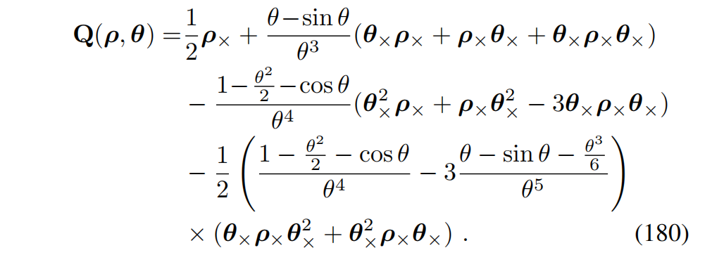
右雅可比及其逆由 (76) 得:
J r ( ρ , θ ) = J l ( − ρ , − θ ) , J r − 1 ( ρ , θ ) = J l − 1 ( − ρ , − θ ) . J_r(\rho, \theta) = J_l(-\rho, -\theta), \quad J_r^{-1}(\rho, \theta) = J_l^{-1}(-\rho, -\theta). Jr(ρ,θ)=Jl(−ρ,−θ),Jr−1(ρ,θ)=Jl−1(−ρ,−θ).
4) 刚体运动作用
刚体对点 p \mathbf{p} p 的作用为:
M ⋅ p = t + R p . (181) M \cdot \mathbf{p} = t + R \mathbf{p}. \tag{181} M⋅p=t+Rp.(181)
因此,当 τ → 0 \tau \to 0 τ→0 时,有 Exp ( τ ) → I + τ ∧ \text{Exp}(\tau) \to I + \tau^\wedge Exp(τ)→I+τ∧,可得
J M M ⋅ p = lim τ → 0 M Exp ( τ ) ⋅ p − M ⋅ p τ = [ R − R [ p ] × ] , (182) J_M^{M \cdot p} = \lim_{\tau \to 0} \frac{M \text{Exp}(\tau) \cdot p - M \cdot p}{\tau} = \begin{bmatrix} R & -R [p]_\times \end{bmatrix}, \tag{182} JMM⋅p=τ→0limτMExp(τ)⋅p−M⋅p=[R−R[p]×],(182)
J p M ⋅ p = R . (183) J^{M \cdot p}_p = R. \tag{183} JpM⋅p=R.(183)
附录 E
平移群 ( R n , + ) (\mathbb{R}^n, +) (Rn,+) 与 T ( n ) T(n) T(n)
群 ( R n , + ) (\mathbb{R}^n, +) (Rn,+) 是向量在加法下的群,可视为平移群。它被认为是平凡的,因为群元素、李代数和切空间都是相同的,因此有 t = t ∧ = Exp ( t ) t = t^\wedge = \text{Exp}(t) t=t∧=Exp(t)。其等价的矩阵群(在乘法下)为平移群 T ( n ) T(n) T(n),其群、李代数和切向量元素为:
T ≜ [ I t 0 1 ] ∈ T ( n ) , t ∧ ≜ [ 0 t 0 0 ] ∈ t ( n ) , t ∈ R n . T \triangleq \begin{bmatrix} I & t \\ 0 & 1 \end{bmatrix} \in T(n), \quad t^\wedge \triangleq \begin{bmatrix} 0 & t \\ 0 & 0 \end{bmatrix} \in t(n), \quad t \in \mathbb{R}^n. T≜[I0t1]∈T(n),t∧≜[00t0]∈t(n),t∈Rn.
等价性可通过观察 T ( 0 ) = I T(0) = I T(0)=I, T ( − t ) = T ( t ) − 1 T(-t) = T(t)^{-1} T(−t)=T(t)−1,以及可交换的复合
T 1 T 2 = [ I t 1 + t 2 0 1 ] T_1 T_2 = \begin{bmatrix} I & t_1 + t_2 \\ 0 &1 & \end{bmatrix} T1T2=[I0t1+t21]
有效地将向量 t 1 t_1 t1 与 t 2 t_2 t2 相加来验证。由于 R n \mathbb{R}^n Rn 中的加法可交换, T ( n ) T(n) T(n) 中的复合乘积也同样可交换。
由于 T ( n ) T(n) T(n) 是 S E ( n ) SE(n) SE(n) 的子群且 R = I R = I R=I,其指数映射可通过取 (156, 172) 中 R = I R = I R=I 并推广到任意 n n n 得到:
Exp : R n → T ( n ) , T = Exp ( t ) = [ I t 0 I ] . (184) \text{Exp} : \mathbb{R}^n \to T(n), \quad T = \text{Exp}(t) = \begin{bmatrix} I & t \\ 0 &I& \end{bmatrix}. \tag{184} Exp:Rn→T(n),T=Exp(t)=[I0tI].(184)
T ( n ) T(n) T(n) 的指数映射也可通过对 exp ( t ∧ ) \exp(t^\wedge) exp(t∧) 的泰勒展开得到,注意到 ( t ∧ ) 2 = 0 (t^\wedge)^2 = 0 (t∧)2=0。这也立即证明了 ( R n , + ) (\mathbb{R}^n, +) (Rn,+) 群的等价指数映射,即恒等映射:
Exp : R n → R n , t = Exp ( t ) . (185) \text{Exp} : \mathbb{R}^n \to \mathbb{R}^n, \quad t = \text{Exp}(t). \tag{185} Exp:Rn→Rn,t=Exp(t).(185)
由此在 R n \mathbb{R}^n Rn 中产生了平凡的、可交换的、左右一致的加法与减法运算符:
t 1 ⊕ t 2 = t 1 + t 2 , (186) t_1 \oplus t_2 = t_1 + t_2, \tag{186} t1⊕t2=t1+t2,(186)
t 2 ⊖ t 1 = t 2 − t 1 . (187) t_2 \ominus t_1 = t_2 - t_1. \tag{187} t2⊖t1=t2−t1.(187)
A. 雅可比块
我们对 T ( n ) T(n) T(n) 和 R n \mathbb{R}^n Rn 的平移统一表示,分别记作 S S S 和 T T T。雅可比矩阵是平凡的(可与 S1 和 SO(2) 的雅可比块 A-C1 对比):
Ad T = I ∈ R n × n , (188) \text{Ad}_T = I \in \mathbb{R}^{n \times n}, \tag{188} AdT=I∈Rn×n,(188)
J T T − 1 = − I ∈ R n × n , (189) J_T^{T^{-1}} = -I \in \mathbb{R}^{n \times n}, \tag{189} JTT−1=−I∈Rn×n,(189)
J T T ∘ S = J T S ∘ S = I ∈ R n × n , (190) J_T^{T \circ S} = J_T^{S \circ S} = I \in \mathbb{R}^{n \times n}, \tag{190} JTT∘S=JTS∘S=I∈Rn×n,(190)
J r = J l = I ∈ R n × n , (191) J_r = J_l = I \in \mathbb{R}^{n \times n}, \tag{191} Jr=Jl=I∈Rn×n,(191)
J T T ⊕ v = J T v ⊕ v = I ∈ R n × n , (192) J_T^{T \oplus v} = J_T^{v \oplus v} = I \in \mathbb{R}^{n \times n}, \tag{192} JTT⊕v=JTv⊕v=I∈Rn×n,(192)
J S S ⊖ T = − J S T ⊖ T = I ∈ R n × n . (193) J_S^{S \ominus T} = -J_S^{T \ominus T} = I \in \mathbb{R}^{n \times n}. \tag{193} JSS⊖T=−JST⊖T=I∈Rn×n.(193)

DAMO开发者矩阵,由阿里巴巴达摩院和中国互联网协会联合发起,致力于探讨最前沿的技术趋势与应用成果,搭建高质量的交流与分享平台,推动技术创新与产业应用链接,围绕“人工智能与新型计算”构建开放共享的开发者生态。
更多推荐

 35
35 0
0- 0


 已为社区贡献17条内容

所有评论(0)