在实际工程和科学研究中，我们经常会遇到这样的问题：有一组散乱的实验数据，想要从中找出规律，建立数学模型。今天就来给大家介绍MATLAB中8种实用的数据拟合方法！

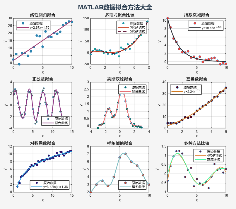
1. 线性回归拟合

最基础的拟合方法，适合线性关系明显的数据。

% 生成线性数据
x = 0:0.5:10;
y = 2.5*x + 1.2 + 2*randn(size(x));

% 线性回归拟合
p = polyfit(x, y, 1);
y_fit = polyval(p, x);

% 绘图
figure('Position', [100, 100, 1000, 800])
subplot(3,3,1)
plot(x, y, 'o', 'MarkerSize', 6, 'MarkerFaceColor', '#2E86AB')
hold on
plot(x, y_fit, '-', 'LineWidth', 2, 'Color', '#A23B72')
grid on
title('线性回归拟合', 'FontSize', 11, 'FontWeight', 'bold')
xlabel('x')
ylabel('y')
legend('原始数据', sprintf('y=%.2fx+%.2f', p(1), p(2)), 'Location', 'northwest')

2. 多项式拟合

适合曲线趋势的数据，可调节多项式阶数。

% 生成曲线数据
x = 0:0.3:8;
y = 0.5*x.^3 - 2*x.^2 + 1.5*x + 3 + 8*randn(size(x));

% 3次多项式拟合
p3 = polyfit(x, y, 3);
y_fit3 = polyval(p3, x);

% 5次多项式拟合
p5 = polyfit(x, y, 5);
y_fit5 = polyval(p5, x);

subplot(3,3,2)
plot(x, y, 'o', 'MarkerSize', 5, 'MarkerFaceColor', '#18A999')
hold on
plot(x, y_fit3, '-', 'LineWidth', 2, 'Color', '#C73E1D')
plot(x, y_fit5, '--', 'LineWidth', 2, 'Color', '#5B0E2D')
grid on
title('多项式拟合比较', 'FontSize', 11, 'FontWeight', 'bold')
xlabel('x')
ylabel('y')
legend('原始数据', '3次多项式', '5次多项式', 'Location', 'northeast')

3. 指数衰减拟合

适合衰减过程、放射性衰变等场景。

% 生成指数衰减数据
x = 0:0.5:10;
y = 10*exp(-0.5*x) + 0.5*randn(size(x));

% 指数拟合
ft = fittype('a*exp(-b*x)', 'independent', 'x');
[fitresult, gof] = fit(x', y', ft, 'StartPoint', [8, 0.3]);

x_fit = linspace(0, 10, 100);
y_fit = fitresult(x_fit);

subplot(3,3,3)
plot(x, y, 'o', 'MarkerSize', 6, 'MarkerFaceColor', '#F24236')
hold on
plot(x_fit, y_fit, '-', 'LineWidth', 2, 'Color', '#2A2D34')
grid on
title('指数衰减拟合', 'FontSize', 11, 'FontWeight', 'bold')
xlabel('x')
ylabel('y')
legend('原始数据', sprintf('y=%.2fe^{-%.2fx}', fitresult.a, fitresult.b), 'Location', 'northeast')

4. 正弦波拟合

适合周期性振动数据。

% 生成正弦波数据
x = 0:0.2:4*pi;
y = 2.5*sin(1.8*x + 0.5) + 0.3*cos(3*x) + 0.4*randn(size(x));

% 正弦拟合
ft = fittype('a*sin(b*x + c) + d*cos(e*x)', 'independent', 'x');
[fitresult, gof] = fit(x', y', ft, 'StartPoint', [2, 2, 0, 0.2, 3]);

x_fit = linspace(0, 4*pi, 200);
y_fit = fitresult(x_fit);

subplot(3,3,4)
plot(x, y, 'o', 'MarkerSize', 4, 'MarkerFaceColor', '#5B6C5D')
hold on
plot(x_fit, y_fit, '-', 'LineWidth', 2, 'Color', '#8F3985')
grid on
title('正弦波拟合', 'FontSize', 11, 'FontWeight', 'bold')
xlabel('x')
ylabel('y')
legend('原始数据', '拟合曲线', 'Location', 'southeast')

5. 高斯拟合

适合正态分布、峰值分析等场景。

% 生成高斯分布数据
x = -3:0.2:3;
y = 2.5*exp(-((x-0.3)/0.8).^2) + 1.2*exp(-((x+1.5)/0.6).^2) + 0.1*randn(size(x));

% 高斯拟合（双峰）
ft = fittype('a1*exp(-((x-b1)/c1)^2) + a2*exp(-((x-b2)/c2)^2)', 'independent', 'x');
[fitresult, gof] = fit(x', y', ft, 'StartPoint', [2, 0, 1, 1, -1.5, 1]);

x_fit = linspace(-3, 3, 200);
y_fit = fitresult(x_fit);

subplot(3,3,5)
plot(x, y, 'o', 'MarkerSize', 5, 'MarkerFaceColor', '#0B6E4F')
hold on
plot(x_fit, y_fit, '-', 'LineWidth', 2, 'Color', '#E56B70')
grid on
title('高斯双峰拟合', 'FontSize', 11, 'FontWeight', 'bold')
xlabel('x')
ylabel('y')
legend('原始数据', '拟合曲线', 'Location', 'northeast')

6. 幂函数拟合

适合幂律关系的数据。

% 生成幂函数数据
x = 1:0.2:5;
y = 2.3*x.^1.7 + 0.8*randn(size(x));

% 幂函数拟合
ft = fittype('a*x^b', 'independent', 'x');
[fitresult, gof] = fit(x', y', ft, 'StartPoint', [2, 1.5]);

x_fit = linspace(1, 5, 100);
y_fit = fitresult(x_fit);

subplot(3,3,6)
plot(x, y, 'o', 'MarkerSize', 6, 'MarkerFaceColor', '#4C061D')
hold on
plot(x_fit, y_fit, '-', 'LineWidth', 2, 'Color', '#D17A22')
grid on
title('幂函数拟合', 'FontSize', 11, 'FontWeight', 'bold')
xlabel('x')
ylabel('y')
legend('原始数据', sprintf('y=%.2fx^{%.2f}', fitresult.a, fitresult.b), 'Location', 'northwest')

7. 对数拟合

适合对数增长或衰减的数据。

% 生成对数数据
x = 1:0.3:15;
y = 3.5*log(x) + 1.2 + 0.4*randn(size(x));

% 对数拟合
ft = fittype('a*log(x) + b', 'independent', 'x');
[fitresult, gof] = fit(x', y', ft, 'StartPoint', [3, 1]);

x_fit = linspace(1, 15, 100);
y_fit = fitresult(x_fit);

subplot(3,3,7)
plot(x, y, 'o', 'MarkerSize', 5, 'MarkerFaceColor', '#3A015C')
hold on
plot(x_fit, y_fit, '-', 'LineWidth', 2, 'Color', '#1E91D6')
grid on
title('对数函数拟合', 'FontSize', 11, 'FontWeight', 'bold')
xlabel('x')
ylabel('y')
legend('原始数据', sprintf('y=%.2fln(x)+%.2f', fitresult.a, fitresult.b), 'Location', 'southeast')

8. 样条插值拟合

适合需要光滑曲线且不需要显式表达式的情况。

% 生成不规则数据
x = [0, 1, 2, 3, 4, 5, 6, 7, 8, 9, 10];
y = [2, 3, 3.5, 2.8, 4, 6.5, 7, 6, 5.5, 4.2, 3];

% 样条插值
x_fit = linspace(0, 10, 100);
y_spline = spline(x, y, x_fit);

subplot(3,3,8)
plot(x, y, 'o', 'MarkerSize', 6, 'MarkerFaceColor', '#BB4430')
hold on
plot(x_fit, y_spline, '-', 'LineWidth', 2, 'Color', '#7EBDC2')
grid on
title('样条插值拟合', 'FontSize', 11, 'FontWeight', 'bold')
xlabel('x')
ylabel('y')
legend('原始数据', '样条曲线', 'Location', 'southeast')

9. 综合比较图

% 创建综合比较图
subplot(3,3,9)
x_demo = 0:0.5:10;
y_demo = 2*sin(0.8*x_demo) .* exp(-0.2*x_demo) + 0.3*randn(size(x_demo));

% 三种不同拟合方法
p_poly = polyfit(x_demo, y_demo, 4);
y_poly = polyval(p_poly, x_demo);

ft_exp = fittype('a*exp(-b*x)*sin(c*x)', 'independent', 'x');
[fit_exp, ~] = fit(x_demo', y_demo', ft_exp, 'StartPoint', [2, 0.2, 1]);
y_exp = fit_exp(x_demo);

% 绘图比较
plot(x_demo, y_demo, 'o', 'MarkerSize', 5, 'MarkerFaceColor', '#6B2737')
hold on
plot(x_demo, y_poly, '-', 'LineWidth', 1.5, 'Color', '#E08E45')
plot(x_demo, y_exp, '-', 'LineWidth', 1.5, 'Color', '#40F99B')
grid on
title('多种方法比较', 'FontSize', 11, 'FontWeight', 'bold')
xlabel('x')
ylabel('y')
legend('原始数据', '4次多项式', '衰减正弦', 'Location', 'northeast')

% 调整布局
sgtitle('MATLAB数据拟合方法大全', 'FontSize', 16, 'FontWeight', 'bold', 'Color', '#2C3E50')

拟合质量评估指标

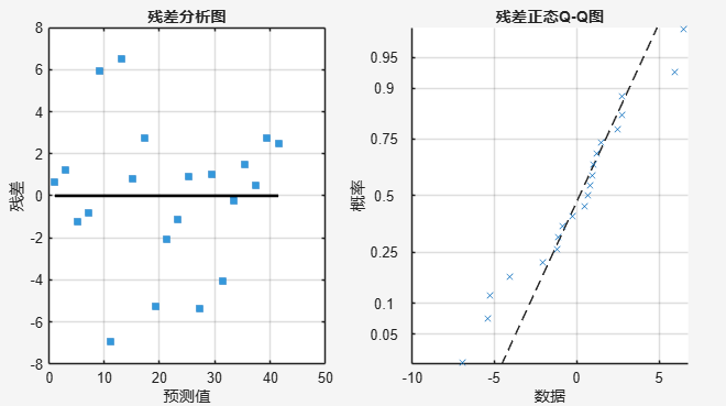
% 计算拟合优度指标
figure('Position', [200, 200, 800, 400])

% 以线性回归为例展示残差分析
x_test = 0:1:20;
y_true = 2*x_test + 1;
y_measured = y_true + 3*randn(size(x_test));

p_test = polyfit(x_test, y_measured, 1);
y_pred = polyval(p_test, x_test);
residuals = y_measured - y_pred;

% 残差图
subplot(1,2,1)
plot(y_pred, residuals, 's', 'MarkerSize', 6, 'MarkerFaceColor', '#3498DB')
hold on
plot([min(y_pred), max(y_pred)], [0, 0], 'k-', 'LineWidth', 2)
xlabel('预测值')
ylabel('残差')
title('残差分析图', 'FontWeight', 'bold')
grid on

% Q-Q图
subplot(1,2,2)
probplot('normal', residuals)
title('残差正态Q-Q图', 'FontWeight', 'bold')
grid on

% 显示拟合优度
R2 = 1 - sum(residuals.^2) / sum((y_measured - mean(y_measured)).^2);
fprintf('确定系数 R² = %.4f\n', R2);