通过一个简单的电商零售数据集,了解数据分析流程
·
目录
数据分析流程
本文通过对一个简单的电商零售数据案例进行粗略分析,介绍做数据分析时的项目流程。(jupyter notebook)
完整项目文件:https://download.csdn.net/download/W_H_M_2018/12338118
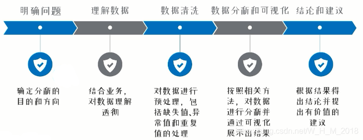
1.数据分析真实项目流程
- 明确问题:明确问题是数据分析中的第一步,必须民却数据分析的真实需求
- 理解数据:数据获取和数据探索
- 数据清洗:一个数据分析项目大部分时间花在数据清洗上。
- 数据分析和可视化:对清洗后的数据进行分析,并且通过可视化展示出结果
- 结论和建议:对结果进行解读,得出有价值的结论且提出相关建议
2.数据分析方法
- 常用统计方法,例如计算常用统计量和构建相关指标
- 图表法,通过各种图形结合来展示数据里面的信息
- 机器学习算法,对于复杂的分析,会涉及到模型构建
3.零售消费数据数据集介绍
数据集下载地址:https://download.csdn.net/download/W_H_M_2018/12337579
该数据来源于kaggle,是一家注册在英国的电子商务网站的2010年12月份-2011年12月份之间的交易数据该公司主要销售独特的全天候礼品,大部分出售对象是批发商。
数据包含541910行,8个字段,字段内容为:
- InvoiceNo: 订单编号,每笔交易有6个整数,退货订单编号开头有字母’C’。
- StockCode: 产品编号,由5个整数组成。
- Description: 产品描述。
- Quantity: 产品数量,有负号的表示退货
- InvoiceDate: 订单日期和时间。
- UnitPrice: 单价(英镑),单位产品的价格。
- CustomerID:客户编号,每个客户编号由5位数字组成。
- Country: 国家的名称,每个客户所在国家/地区的名称。
4.分析内容
明确分析的目的
- 购买商品前十的国家是?
- 交易额前十的国家是?
- 哪些月份销售较佳?
- 客单价多少?
- 用户消费行为分析
案例分析实战
1理解数据
import pandas as pd
import matplotlib.pyplot as plt
import os
import numpy as np

import plotly as py
import plotly.graph_objs as go
py.offline.init_notebook_mode()
pyplot = py.offline.iplot

os.chdir(r'C:\Users\W\Desktop')

online_data = pd.read_csv('data.csv',encoding = 'ISO-8859-1',dtype = {'CustomerID':str})
online_data.head()
online_data.info()<class 'pandas.core.frame.DataFrame'>
RangeIndex: 541909 entries, 0 to 541908
Data columns (total 8 columns):
InvoiceNo 541909 non-null object
StockCode 541909 non-null object
Description 540455 non-null object
Quantity 541909 non-null int64
InvoiceDate 541909 non-null object
UnitPrice 541909 non-null float64
CustomerID 406829 non-null object
Country 541909 non-null object
dtypes: float64(1), int64(1), object(6)
memory usage: 33.1+ MB查看退货订单
online_data[online_data['InvoiceNo'].str[0]=='C']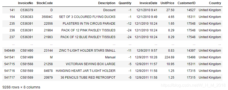
2数据清洗
CustomerID 缺失率较高
# 数据缺失率
online_data.apply(lambda x:sum(x.isnull())/len(x),axis=0)
InvoiceNo 0.000000
StockCode 0.000000
Description 0.002683
Quantity 0.000000
InvoiceDate 0.000000
UnitPrice 0.000000
CustomerID 0.249267
Country 0.000000
dtype: float64删除带有空值的行
# 防止修改df1对online_data造成修改,使用copy对数据做一份拷贝
df1 = online_data.dropna(how='any').copy()

df1.head()
# 将订单日期由字符串转换为标准日期格式
# errors = 'coerce' 错误转换为缺失值(容错处理)
df1['InvoiceDate'] = pd.to_datetime(df1['InvoiceDate'],errors = 'coerce')
# 提取日期部分
df1['InvoiceDate'] = df1['InvoiceDate'].dt.date
df1.head()
# 再次转换日期格式 object->datetime64[ns]
# df1['InvoiceDate'] = pd.to_datetime(df1['InvoiceDate'],errors = 'coerce')
df1.info()
<class 'pandas.core.frame.DataFrame'>
Int64Index: 406829 entries, 0 to 541908
Data columns (total 8 columns):
InvoiceNo 406829 non-null object
StockCode 406829 non-null object
Description 406829 non-null object
Quantity 406829 non-null int64
InvoiceDate 406829 non-null object
UnitPrice 406829 non-null float64
CustomerID 406829 non-null object
Country 406829 non-null object
dtypes: float64(1), int64(1), object(6)
memory usage: 27.9+ MB销售金额
df1['Price'] = df1.apply(lambda x:x[3]*x[5],axis=1)
df1.head()
3数据分析和可视化
1.购买商品前十的国家是?
quantity_first_10 = df1[df1['Quantity']>0].groupby('Country').sum()['Quantity'].sort_values(ascending=False).head(10)
print(quantity_first_10)
Country
United Kingdom 4269472
Netherlands 200937
EIRE 140525
Germany 119263
France 111472
Australia 84209
Sweden 36083
Switzerland 30083
Spain 27951
Japan 26016
Name: Quantity, dtype: int64trace_basic = [go.Bar(x = quantity_first_10.index.tolist(),
y = quantity_first_10.values.tolist(),
marker = dict(color = 'red'),
opacity = .5)]
layout = go.Layout(title = '购买商品前十的国家',xaxis = dict(title='国家'))
figure_basic = go.Figure(data = trace_basic,layout = layout)
pyplot(figure_basic)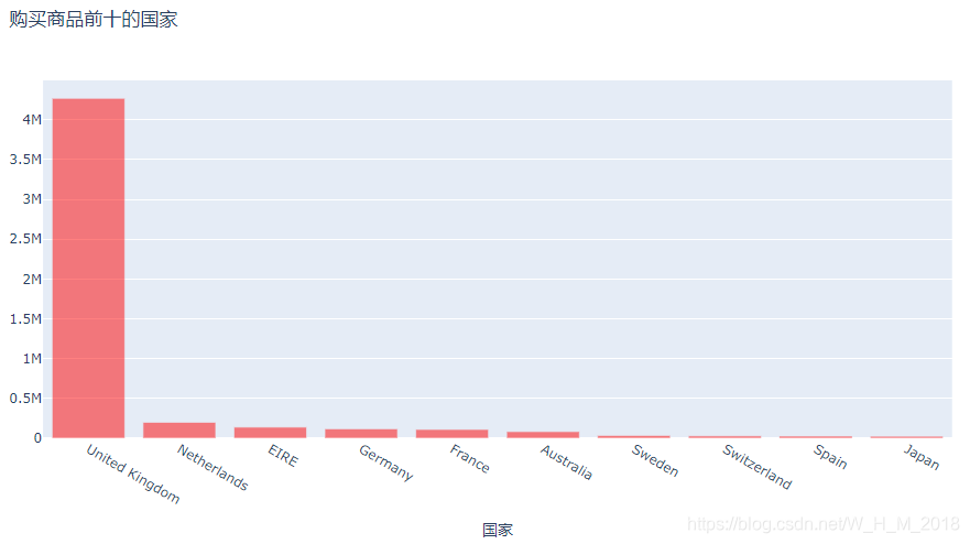
2.交易额前十的国家是?
price_first_10 = df1[df1['Quantity']>0].groupby('Country').sum()['Price'].sort_values(ascending=False).head(10)
print(quantity_first_10)
Country
United Kingdom 4269472
Netherlands 200937
EIRE 140525
Germany 119263
France 111472
Australia 84209
Sweden 36083
Switzerland 30083
Spain 27951
Japan 26016
Name: Quantity, dtype: int64trace_basic = [go.Bar(x = price_first_10.index.tolist(),
y = price_first_10.values.tolist(),
marker = dict(color = 'red'),
opacity = .5)]
layout = go.Layout(title = '交易额前十的国家',xaxis = dict(title='国家'))
figure_basic = go.Figure(data = trace_basic,layout = layout)
pyplot(figure_basic)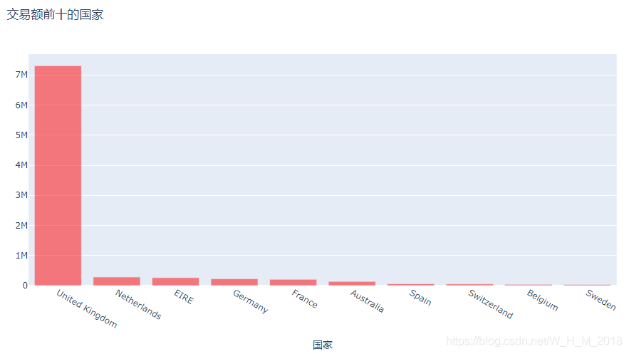
3.哪些月份销售较佳?
df1.head()
df1['month'] = pd.to_datetime(df1['InvoiceDate'],errors = 'coerce').dt.month

df1.head()
month_quantity = df1[df1['Quantity']>0].groupby('month').sum()['Quantity'].sort_values(ascending=False)
print(month_quantity)
month
11 681888
12 599693
10 593908
9 544899
8 398938
5 373685
7 369432
6 363699
1 349147
3 348544
4 292225
2 265638
Name: Quantity, dtype: int64seaborn 绘图更简便
import seaborn as sns
sns.set(style = 'darkgrid',context='notebook',font_scale=1.2)

month_quantity.plot(kind='bar')
plt.xticks(rotation=45) #标签旋转45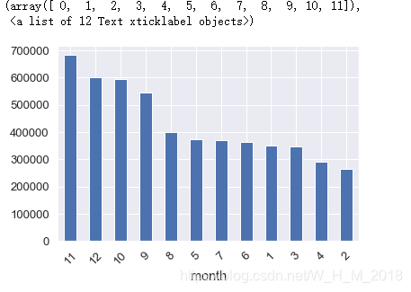
4.客单价多少?
三种维度
sumPrice = df1[df1['Quantity']>0]['Price'].sum()
sumPrice8911407.9041.按每次订单
#订单有重复 未去重
sum_InvoiceNo = df1[df1['Quantity']>0]['InvoiceNo'].count()
sum_InvoiceNo397924avgPrice = sumPrice/sum_InvoiceNo
avgPrice22.3947485047395962.按每个订单
# 去除重复订单号
sum_InvoiceNo = df1[df1['Quantity']>0]['InvoiceNo'].drop_duplicates().count()
sum_InvoiceNo18536avgPrice = sumPrice/sum_InvoiceNo
avgPrice480.76218731117823.按每个客户
# 客单价
sum_CustomerID = df1[df1['Quantity']>0]['CustomerID'].drop_duplicates().count()
sum_CustomerID4339avgPrice = sumPrice/sum_CustomerID
avgPrice2053.79301774602445.用户消费行为分析
customer = df1[df1['Quantity']>0].groupby('CustomerID').agg({'InvoiceNo':'nunique',
                                                           'Quantity':np.sum,
                                                           'Price':np.sum})
customer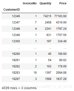
customer.describe()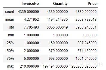
结论和建议
- 用户平均消费4次,有的客户甚至消费高达210次,是产品的忠诚客户
- 用户平均消费金额为2053元,而75%的用户消费金额只有1661,可见,有些用户消费金额较大,属于非常有价值的用户,需要重点保持关注
- 用户购买产品数量平均高达1194件,由于销售对象主要是批发商,算是正常的数量数

DAMO开发者矩阵,由阿里巴巴达摩院和中国互联网协会联合发起,致力于探讨最前沿的技术趋势与应用成果,搭建高质量的交流与分享平台,推动技术创新与产业应用链接,围绕“人工智能与新型计算”构建开放共享的开发者生态。
更多推荐



 4
4 0
0- 0


 已为社区贡献3条内容

所有评论(0)