import warnings
warnings.filterwarnings('ignore')
import missingno as msno
import pandas as pd
from pandas import DataFrame
import matplotlib.pyplot as plt 
import seaborn as sns
import numpy as np

import pandas as pd
from pandas import DataFrame, Series
import matplotlib.pyplot as plt 

path = '../data/tianchi/'
# .read_csv返回DataFrame形式的数据
train = pd.read_csv(path+'train.csv')
test = pd.read_csv(path+'testA.csv')

# 1首先要看下数据集的分布情况
train.head().append(train.tail())

	id	heartbeat_signals	label
0	0	0.9912297987616655,0.9435330436439665,0.764677...	0.0
1	1	0.9714822034884503,0.9289687459588268,0.572932...	0.0
2	2	1.0,0.9591487564065292,0.7013782792997189,0.23...	2.0
3	3	0.9757952826275774,0.9340884687738161,0.659636...	0.0
4	4	0.0,0.055816398940721094,0.26129357194994196,0...	2.0
99995	99995	1.0,0.677705342021188,0.22239242747868546,0.25...	0.0
99996	99996	0.9268571578157265,0.9063471198026871,0.636993...	2.0
99997	99997	0.9258351628306013,0.5873839035878395,0.633226...	3.0
99998	99998	1.0,0.9947621698382489,0.8297017704865509,0.45...	2.0
99999	99999	0.9259994004527861,0.916476635326053,0.4042900...	0.0

test.head().append(test.tail())

	id	heartbeat_signals
0	100000	0.9915713654170097,1.0,0.6318163407681274,0.13...
1	100001	0.6075533139615096,0.5417083883163654,0.340694...
2	100002	0.9752726292239277,0.6710965234906665,0.686758...
3	100003	0.9956348033996116,0.9170249621481004,0.521096...
4	100004	1.0,0.8879490481178918,0.745564725322326,0.531...
19995	119995	1.0,0.8330283177934747,0.6340472606311671,0.63...
19996	119996	1.0,0.8259705825857048,0.4521053488322387,0.08...
19997	119997	0.951744840752379,0.9162611283848351,0.6675251...
19998	119998	0.9276692903808186,0.6771898159607004,0.242906...
19999	119999	0.6653212231837624,0.527064114047737,0.5166625...

# 2,利用describel()和info()总揽数据分布和数据类型
# 个数count、平均值mean、方差std、最小值min、中位数25% 50% 75% 、以及最大值
train.describe()

	id	label
count	100000.000000	100000.000000
mean	49999.500000	0.856960
std	28867.657797	1.217084
min	0.000000	0.000000
25%	24999.750000	0.000000
50%	49999.500000	0.000000
75%	74999.250000	2.000000
max	99999.000000	3.000000

test.describe()

	id
count	20000.000000
mean	109999.500000
std	5773.647028
min	100000.000000
25%	104999.750000
50%	109999.500000
75%	114999.250000
max	119999.000000

train.info()

<class 'pandas.core.frame.DataFrame'>
RangeIndex: 100000 entries, 0 to 99999
Data columns (total 3 columns):
 #   Column             Non-Null Count   Dtype  
---  ------             --------------   -----  
 0   id                 100000 non-null  int64  
 1   heartbeat_signals  100000 non-null  object 
 2   label              100000 non-null  float64
dtypes: float64(1), int64(1), object(1)
memory usage: 2.3+ MB

test.info()

<class 'pandas.core.frame.DataFrame'>
RangeIndex: 20000 entries, 0 to 19999
Data columns (total 2 columns):
 #   Column             Non-Null Count  Dtype 
---  ------             --------------  ----- 
 0   id                 20000 non-null  int64 
 1   heartbeat_signals  20000 non-null  object
dtypes: int64(1), object(1)
memory usage: 312.6+ KB

# 3,缺失值判断
train.isnull().sum()

id                   0
heartbeat_signals    0
label                0
dtype: int64

test.isnull().sum()

id                   0
heartbeat_signals    0
dtype: int64

# 4,查看分布情况
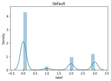
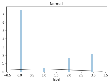
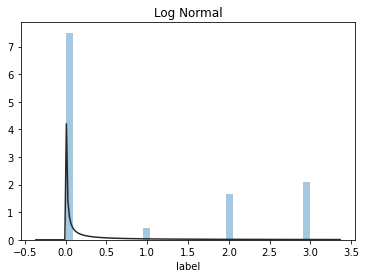
## 1) 总体分布概况（无界约翰逊分布等）
import scipy.stats as st
y = train['label']
plt.figure(1); plt.title('Default')
sns.distplot(y, rug=True, bins=20)
plt.figure(2); plt.title('Normal')
sns.distplot(y, kde=False, fit=st.norm)
plt.figure(3); plt.title('Log Normal')
sns.distplot(y, kde=False, fit=st.lognorm)

<matplotlib.axes._subplots.AxesSubplot at 0x199f1cf9948>

# 2）查看skewness and kurtosis
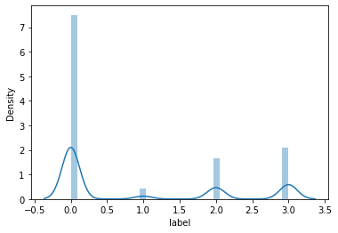
sns.distplot(train['label']);
print("Skewness: %f" % train['label'].skew())
print("Kurtosis: %f" % train['label'].kurt())

Skewness: 0.871005
Kurtosis: -1.009573

train.skew(), train.kurt()

(id       0.000000
 label    0.871005
 dtype: float64,
 id      -1.200000
 label   -1.009573
 dtype: float64)

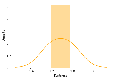
sns.distplot(train.kurt(),color='orange',axlabel ='Kurtness')

<matplotlib.axes._subplots.AxesSubplot at 0x199f1f40688>

## 3) 查看预测值的具体频数
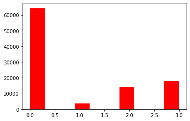
plt.hist(train['label'], orientation = 'vertical',histtype = 'bar', color ='red')
plt.show()