在此之前，我们主要关注的是定位，即稀疏路标点主要用于计算相机位姿，但是仅有稀疏特征点显然是不够的，机器人无法得知哪里是桌子、哪里是墙，无法进行导航和避障。因此在这一讲，主要目标是构建稠密地图

单目稠密重建

极线搜索与块匹配

回顾一下视觉里程计 1 中对极几何的内容，极线搜索其实和三角测量的思路很像

极线搜索

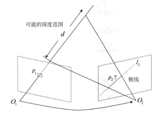
假设我们在第一帧看到一个特征点 $p_1$，由于此时我们并不知道其深度，所以它对应的空间点 $P$ 可能在一条射线的任意一点上
在第二帧中，这条射线的投影就是一条线，即极线。那么第二帧中的匹配点，必然落在极线上，只需在极线上搜索就能找到 $p_2$

必须知道相机之间的运动，否则无法确定极线

块匹配

现在问题来到了如何快速确定 $p_2$ ，由于单个像素的灰度值可区分度太低了，我们可以在 $p_1$ 周围取一个像素块，并在极线上取一个同样大小的像素块滑动，寻找最相似的方块。需要注意的是，只有假设整个小块的灰度值不变，比较才有意义

相似度衡量指标：

• SAD：绝对差之和。计算简单，速度快
  $$S(A,B{)}_{SAD}=\sum _{i,j}|A(i,j)-B(i,j)|$$
• SSD：平方差之和。对大误差敏感
  $$S(A,B{)}_{SSD}=\sum _{i,j}(A(i,j)-B(i,j){)}^2$$
• NCC：归一化互相关。计算复杂，但是鲁棒性强（相似度，接近 1 表示相似）
  $$S(A,B{)}_{NCC}=\frac{{\sum }_{i,j}A(i,j)B(i,j)}{\sqrt{{\sum }_{i,j}A(i,j{)}^2{\sum }_{i,j}B(i,j{)}^2}}$$

假设现在使用 NCC 进行相似性度量，可以得到类似数据

![[NCC.png]]

该分布存在多个峰值，所以一般倾向于使用概率分布而非单一数值描述深度

深度滤波器

假设深度的分布服从高斯分布
$$P(d)\sim N(\mu ,{\sigma }^2)$$

• $\mu$（均值）：要估计的深度值
• ${\sigma }^2$（方差）：深度值的不程度

接下来我们要解决的问题是一个信息融合问题，假设新观测的信息也满足高斯分布，随着相机的不断移动，我们不断把新的观测融合到现有的高斯分布中，使其向收敛靠近

已知两个高斯分布的乘积仍为高斯分布，有
$${\mu }_{fuse}=\frac{{\sigma }_{obs}^2\mu +{\sigma }^2{\mu }_{obs}}{{\sigma }^2+{\sigma }_{obs}^2},{\sigma }_{fuse}^2=\frac{{\sigma }^2{\sigma }_{obs}^2}{{\sigma }^2+{\sigma }_{obs}^2}$$
仅考虑几何不确定性，已知 $p_1$ 和 $p_2$ 对应，由此观测到 $p_1$ 的深度值，求得对应的三维点 $P$ 。现在假设极线 $l_2$ 存在一个像素的误差，那么最终求得的三维点 $P$ ，误差会有多大呢？

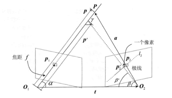
推导的过程就略掉了，直接给出答案
$$||p^{\prime }||=||t||\frac{\sin {\beta }^{\prime }}{\sin {\gamma }^{\prime }}$$
此时可以设
$${\sigma }_{obs}=||p||-||p^{\prime }||$$
当不确定性小于某个阈值时，则可以认为深度数据已经收敛

单目稠密建图代码实现

#include <opencv2/opencv.hpp>
#include <iostream>
#include <sophus/se3.hpp>
#include <Eigen/Core>
#include <fstream>

// parameters
const int boarder = 20;  // 边缘宽度
const int width = 640;   // 图像宽度
const int height = 480;  // 图像高度
const double fx = 481.2f;
const double fy = -480.0f;
const double cx = 319.5f;
const double cy = 239.5f;
const int ncc_windows_size = 3;  // NCC窗口半宽度
const int ncc_area = (2 * ncc_windows_size + 1) * (2 * ncc_windows_size + 1);  // NCC窗口面积
const double min_cov = 0.1;  // 最小方差
const double max_cov = 10;   // 最大方差

/**
  @brief 使用新图像更新深度图
  @param ref 参考图像
  @param curr 当前图像
  @param T 从参考图像到当前图像的位姿变换
  @param depth 深度图
  @param depth_cov 深度协方差图
  @return 是否更新成功
 */
bool update(const cv::Mat& ref, const cv::Mat& curr, const Sophus::SE3d& T, cv::Mat& depth, cv::Mat& depth_cov2);

/**
 * @brief 进行极线搜索
 * @param ref 参考图像
 * @param curr 当前图像
 * @param T 从参考图像到当前图像的位姿变换
 * @param pt_ref 参考图像中的点
 * @param depth_mu 深度均值
 * @param depth_cov 深度协方差
 * @param pt_curr 当前图像中的点
 * @param epipolar_direaction 极线方向
 */
bool epipolarSearch(const cv::Mat& ref, const cv::Mat& curr, const Sophus::SE3d& T, const Eigen::Vector2d& pt_ref, const double& depth_mu, const double& depth_cov, Eigen::Vector2d& pt_curr, Eigen::Vector2d& epipolar_direaction);

/**
 * @brief 更新深度滤波器
 * @param pt_ref 参考图像中的点
 * @param pt_curr 当前图像中的点
 * @param T 从参考图像到当前图像的位姿变换
 * @param epipolar_direction 极线方向
 * @param depth 深度均值
 * @param depth_cov2 深度方差
 * @return 是否更新成功
 */
bool updateDepthFilter(const Eigen::Vector2d& pt_ref, const Eigen::Vector2d& pt_curr, const Sophus::SE3d& T, const Eigen::Vector2d& epipolar_direction, cv::Mat& depth, cv::Mat& depth_cov2);

/**
 * @brief 计算 NCC
 * @param ref 参考图像
 * @param curr 当前图像
 * @param pt_ref 参考图像中的点
 * @param pt_curr 当前图像中的点
 * @return NCC值
 */
double NCC(const cv::Mat& ref, const cv::Mat& curr, const Eigen::Vector2d& pt_ref, const Eigen::Vector2d& pt_curr);

// 双线性灰度插值
inline double getBilinearInterpolatedValue(const cv::Mat& img, const Eigen::Vector2d& pt)
{
    const uchar* data = &img.data[int(pt(1, 0)) * img.step + int(pt(0, 0))];
    double xx = pt(0, 0) - floor(pt(0, 0));
    double yy = pt(1, 0) - floor(pt(1, 0));
    return ((1 - xx) * (1 - yy) * double(data[0]) + xx * (1 - yy) * double(data[1]) + 
            (1 - xx) * yy * double(data[img.step]) + xx * yy * double(data[img.step + 1])) / 255.0;
}

// ============================
// 显示估计的深度图
void plotDepth(const cv::Mat& depth_truth, const cv::Mat& depth_estimate);

// 像素转相机坐标系
inline Eigen::Vector3d px2cam(const Eigen::Vector2d px)
{
    return Eigen::Vector3d((px(0, 0) - cx) / fx, (px(1, 0) - cy) / fy, 1);
}

// 相机坐标系转像素
inline Eigen::Vector2d cam2px(const Eigen::Vector3d p_cam)
{
    return Eigen::Vector2d(p_cam(0, 0) * fx / p_cam(2, 0) + cx, p_cam(1, 0) * fy / p_cam(2, 0) + cy);
}

// 判断像素点是否在图像内
inline bool inside(const Eigen::Vector2d& px)
{
    return px(0, 0) >= boarder && px(0, 0) < width - boarder && px(1, 0) >= boarder && px(1, 0) < height - boarder;
}

// 显示极线匹配
void showEpipolarMatch(const cv::Mat& ref, const cv::Mat& curr, const Eigen::Vector2d& px_ref, const Eigen::Vector2d& px_curr);

// 显示极线
void showEpipolarLine(const cv::Mat& ref, const cv::Mat& curr, const Eigen::Vector2d& px_ref, const Eigen::Vector2d& px_min_curr, const Eigen::Vector2d& px_max_curr);

// 评测深度估计
void evaluateDepth(const cv::Mat& depth_truth, const cv::Mat& depth_estimate);
// ============================


bool update(const cv::Mat& ref, const cv::Mat& curr, const Sophus::SE3d& T, cv::Mat& depth, cv::Mat& depth_cov2)
{
    // 从边缘开始遍历每个像素
    for (int x = boarder; x < width - boarder; x++)
    {
        for (int y = boarder; y < height - boarder; y++)
        {
            // 深度收敛或发散
            if (depth_cov2.ptr<double>(y)[x] < min_cov || depth_cov2.ptr<double>(y)[x] > max_cov)
                continue;

            Eigen::Vector2d pt_curr;
            Eigen::Vector2d epipolar_direction;
            bool ret = epipolarSearch(ref, curr, T, Eigen::Vector2d(x, y), depth.ptr<double>(y)[x], sqrt(depth_cov2.ptr<double>(y)[x]), pt_curr, epipolar_direction);
            
            if (ret == false) 
                continue;

            // showEpipolarMatch(ref, curr, Eigen::Vector2d(x, y), pt_curr);
                
            updateDepthFilter(Eigen::Vector2d(x, y), pt_curr, T, epipolar_direction, depth, depth_cov2);
        }
    }

    return true;
}

bool epipolarSearch(const cv::Mat& ref, const cv::Mat& curr, const Sophus::SE3d& T, const Eigen::Vector2d& pt_ref, const double& depth_mu, const double& depth_cov, Eigen::Vector2d& pt_curr, Eigen::Vector2d& epipolar_direaction)
{
    Eigen::Vector3d f_ref = px2cam(pt_ref);
    f_ref.normalize();
    Eigen::Vector3d P_ref = f_ref * depth_mu;  // 3d 点在参考帧下的坐标

    Eigen::Vector2d px_mean_curr = cam2px(T * P_ref);  // 3d 点在当前帧下的像素坐标
    double d_min = depth_mu - 3 * depth_cov, d_max = depth_mu + 3 * depth_cov;  // 深度范围在mu±3sigma内

    if (d_min < 0.1)
        d_min = 0.1;

    Eigen::Vector2d px_min_curr = cam2px(T * (f_ref * d_min));
    Eigen::Vector2d px_max_curr = cam2px(T * (f_ref * d_max));

    Eigen::Vector2d epipolar_line = px_max_curr - px_min_curr;  // 极线
    epipolar_direaction = epipolar_line;                        // 极线方向
    epipolar_direaction.normalize();

    double half_length = 0.5 * epipolar_line.norm();
    if (half_length > 100)
        half_length = 100;

    // showEpipolarLine(ref, curr, pt_ref, px_min_curr, px_max_curr);

    // 在极线上搜索最佳匹配点
    double best_ncc = -1.0;
    Eigen::Vector2d best_px_curr;

    for (double l = -half_length; l <= half_length; l += 0.7)
    {
        Eigen::Vector2d px_curr = px_mean_curr + l * epipolar_direaction;  // 待匹配点
        if (!inside(px_curr))
            continue;   

        double ncc = NCC(ref, curr, pt_ref, px_curr);
        if (ncc > best_ncc)
        {
            best_ncc = ncc;
            best_px_curr = px_curr;
        }
    }

    if (best_ncc < 0.85f)
        return false;

    pt_curr = best_px_curr;
    return true;
}

double NCC(const cv::Mat& ref, const cv::Mat& curr, const Eigen::Vector2d& pt_ref, const Eigen::Vector2d& px_curr)
{
    double mean_ref = 0, mean_curr = 0;
    std::vector<double> values_ref, values_curr;

    for (int x = -ncc_windows_size; x <= ncc_windows_size; x++)
    {
        for (int y = -ncc_windows_size; y <= ncc_windows_size; y++)
        {
            double value_ref = double(ref.ptr<uchar>(int(y + pt_ref(1, 0)))[int(x + pt_ref(0, 0))]) / 255.0;
            mean_ref += value_ref;

            double value_curr = getBilinearInterpolatedValue(curr, Eigen::Vector2d(px_curr(0, 0) + x, px_curr(1, 0) + y));
            mean_curr += value_curr;

            values_ref.push_back(value_ref);
            values_curr.push_back(value_curr);
        }
    }

    mean_ref /= ncc_area;
    mean_curr /= ncc_area;

    // 计算 NCC
    double numerator = 0, demoninator1 = 0, denominator2 = 0;
    for (int i = 0; i < values_ref.size(); i++)
    {
        double n = (values_ref[i] - mean_ref) * (values_curr[i] - mean_curr);
        numerator += n;
        demoninator1 += (values_ref[i] - mean_ref) * (values_ref[i] - mean_ref);
        denominator2 += (values_curr[i] - mean_curr) * (values_curr[i] - mean_curr);
    }

    return numerator / sqrt(demoninator1 * denominator2 + 1e-10);
}

bool updateDepthFilter(const Eigen::Vector2d& px_ref, const Eigen::Vector2d& px_curr, const Sophus::SE3d& T, const Eigen::Vector2d& epipolar_direction, cv::Mat& depth, cv::Mat& depth_cov2)
{
    // 三角化计算深度
    // 这里的 T 是参考帧 -> 当前帧的变换， 需要取逆
    Sophus::SE3d T_inv = T.inverse();
    
    Eigen::Vector3d f_ref = px2cam(px_ref);
    f_ref.normalize();
    Eigen::Vector3d f_curr = px2cam(px_curr);
    f_curr.normalize();

    // d_ref * f_ref = d_curr * (R * f_curr) + t
    // Rf = R * f_curr
    // 构建误差 e = d_ref * f_ref - d_curr * RF - t
    // 令误差最小，构建方程
    // [f_ref^T  - f_ref^T * Rf][d_ref] = [f_ref^T * t]
    // [Rf^T * f_ref, -Rf^T * Rf][d_curr]   [Rf^T * t]
    Eigen::Vector3d t = T_inv.translation(); 
    Eigen::Vector3d Rf = T_inv.so3() * f_curr;
    Eigen::Vector2d b = Eigen::Vector2d(t.dot(f_ref), t.dot(Rf));
    Eigen::Matrix2d A;
    A(0, 0) = f_ref.dot(f_ref);
    A(0, 1) = -f_ref.dot(Rf);
    A(1, 0) = -A(0, 1);
    A(1, 1) = -Rf.dot(Rf);
    Eigen::Vector2d ans = A.inverse() * b;
    Eigen::Vector3d x1 = ans[0] * f_ref;       // 参考帧下的3d点
    Eigen::Vector3d x2 = t + ans[1] * Rf;      // 当前帧下的3d点
    Eigen::Vector3d min_pt = (x1 + x2) / 2.0;
    double depth_estimate = min_pt.norm();

    // 计算深度不确定性
    Eigen::Vector3d p = f_ref * depth_estimate;
    Eigen::Vector3d a = p - t;
    double t_norm = t.norm();
    double a_norm = a.norm();
    double alpha = acos(f_ref.dot(t) / t_norm);
    double beta = acos(-a.dot(t) / (a_norm * t_norm));
    Eigen::Vector3d f_curr_prime = px2cam(px_curr + epipolar_direction);
    f_curr_prime.normalize();
    double beta_prime = acos(f_curr_prime.dot(-t) / t_norm);
    double gamma = M_PI - alpha - beta_prime;
    double p_prime = t_norm * sin(beta_prime) / sin(gamma);
    double d_cov = p_prime - depth_estimate;
    double d_cov2 = d_cov * d_cov;
    
    // 高斯融合
    double mu = depth.ptr<double>(int(px_ref(1, 0)))[int(px_ref(0, 0))];
    double sigma2 = depth_cov2.ptr<double>(int(px_ref(1, 0)))[int(px_ref(0, 0))];

    double mu_fuse = (d_cov2 * mu + sigma2 * depth_estimate) / (sigma2 + d_cov2);
    double sigma2_fuse = (sigma2 * d_cov2) / (sigma2 + d_cov2);

    depth.ptr<double>(int(px_ref(1, 0)))[int(px_ref(0, 0))] = mu_fuse;
    depth_cov2.ptr<double>(int(px_ref(1, 0)))[int(px_ref(0, 0))] = sigma2_fuse;

    return true;
}

bool readDatasetFiles(const std::string& path, std::vector<std::string>& color_image_files, std::vector<Sophus::SE3d>& poses, cv::Mat& ref_depth)
{
    std::ifstream fin(path + "/first_200_frames_traj_over_table_input_sequence.txt"); 
    if (!fin)
    {
        std::cerr << "cannot find the pose file!" << std::endl;
        return false;
    }

    while (!fin.eof())
    {
        std::string image;
        fin >> image;
        double data[7];
        for (double& d : data)
            fin >> d;
        
        color_image_files.push_back(path + "/images/" + image);
        poses.emplace_back(Sophus::SE3d(Eigen::Quaterniond(data[6], data[3], data[4], data[5]), Eigen::Vector3d(data[0], data[1], data[2])));
        if (!fin.good())
            break;
    }

    fin.close();

    // load reference depth
    fin.open(path + "/depthmaps/scene_000.depth");
    ref_depth = cv::Mat(height, width, CV_64F);

    if (!fin)
        return false;

    for (int y = 0; y < height; y++)
    {
        for (int x = 0; x < width; x++)
        {
            double depth = 0;
            fin >> depth;
            ref_depth.ptr<double>(y)[x] = depth / 100.0;
        }
    }

    return true;
}

int main()
{
    std::vector<std::string> color_image_files;
    std::vector<Sophus::SE3d> poses;
    cv::Mat ref_depth;
    bool ret = readDatasetFiles("../data/test_data", color_image_files, poses, ref_depth);
    if (ret == false)
        return -1;

    cv::Mat ref = cv::imread(color_image_files[0], cv::IMREAD_GRAYSCALE);
    Sophus::SE3d pose_ref = poses[0];
    double init_depth = 3.0;
    double init_cov2 = 3.0;
    cv::Mat depth = cv::Mat(height, width, CV_64F, init_depth);        // 初始深度均值
    cv::Mat depth_cov2 = cv::Mat(height, width, CV_64F, init_cov2);   // 初始深度方差

    for (int idx = 1; idx < color_image_files.size(); idx++)
    {
        std::cout << "==== loop ==== " << idx << std::endl;
        cv::Mat curr = cv::imread(color_image_files[idx], cv::IMREAD_GRAYSCALE);
        if (curr.data == nullptr)
            continue;
        Sophus::SE3d pose_curr = poses[idx];
        Sophus::SE3d T_curr_ref = pose_curr.inverse() * pose_ref;
        update(ref, curr, T_curr_ref, depth, depth_cov2);
        evaluateDepth(ref_depth, depth);
        plotDepth(ref_depth, depth);
        cv::imshow("current", curr);
        cv::waitKey(1);
    }

    std::cout << "estimation finished." << std::endl;
    cv::imwrite("depth_estimate.png", depth * 100);
    return 0;   
}

void evaluateDepth(const cv::Mat &depth_truth, const cv::Mat &depth_estimate)
 {
    double ave_depth_error = 0;         // 平均误差
    double ave_depth_error_sq = 0;      // 平方误差
    int cnt_depth_data = 0;
    for (int y = boarder; y < depth_truth.rows - boarder; y++)
    {
        for (int x = boarder; x < depth_truth.cols - boarder; x++) 
        {
            double error = depth_truth.ptr<double>(y)[x] - depth_estimate.ptr<double>(y)[x];
            ave_depth_error += error;
            ave_depth_error_sq += error * error;
            cnt_depth_data++;
        }
    }
    ave_depth_error /= cnt_depth_data;
    ave_depth_error_sq /= cnt_depth_data;

    std::cout << "Average squared error = " << ave_depth_error_sq << ", average error: " << ave_depth_error << std::endl;
}

像素梯度

这里其实可以很直观的看到纯视觉信息的弊端：依赖于纹理信息。对于诸如杂志，花纹等纹理丰富的目标，视觉信息往往可以推理出较为准确的深度信息；但是对于墙壁等梯度不明显的像素，在块匹配时没有区分性，很容易出现误匹配。

同时，像素梯度也和极线方向相关，当像素梯度和极线方向平行时，沿着加息那做块匹配时，我们可以很明显地判断出匹配度最高点在何处，反而当像素梯度与极线方向平行时，处处的匹配度都是相等的，因此无法得到有效匹配

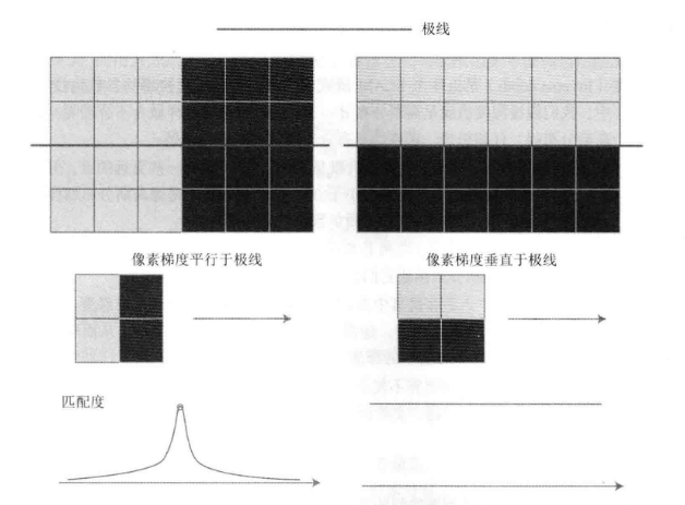
当然，现实往往极线和像素深度的关系不会如此极端，而是偏向于交叉，但是二者关系确切也可做一个算法参考方向

逆深度

既然像素深度无法确定，那么我们是否可以假设其为高斯分布呢？从参数化的角度看，对于三维世界点，我们常用 $x,y,z$ 三个量来描述，但在 SLAM 系统中，通常使用像素坐标 $u,v$ 和深度值 $d$ 来描述三维点。虽然描述的是同一个量，但是前者三个变量的误差是高度耦合的，反映到协方差矩阵中会表现处非对角线元素不为零；而如果使用 $u,v,d$ ，最起码 $u,v$ 和 $d$ 之间是独立的，而且 $u,v$ 通常是确定的，这就可以讲问题简化为一个一维更新问题

此时假设深度值满足高斯分布 $d\sim N(\mu ,{\sigma }^2)$ ，那么问题又来了，如果在室外场景，可能存在距离非常远乃至无穷远处的点，高斯分布难以涵盖这些点。因此，逆深度的用处就彰显出来了，通过对深度取倒数， 原本无穷远处的点将被近似于0，此时深度值可以用高斯分布表示

图像间的变换

做块匹配时，我们假设图像小块在相机运动时保持不变，这个假设在相机平移时是成立的，但当相机发生明显旋转的时候，相关性就会立刻跑偏

因此，在块匹配之前通常要进行一些预处理操作。根据相机模型，如果已知参考帧的一个像素 $P_R$ ，对应的真实三维点世界坐标 $P_W$ 及其深度 $d_R$ ，那么
$$d_R{P}_R=K(R_{RW}{P}_W+t_{RW})$$
在当前帧，也有着同样的变换，故$$d_c{P}_c=d_{R}K{R}_{CW}{R}_{RW}^T{K}^{-1}{P}_R+K{t}_{CW}-K{R}_{CW}{R}_{RW}^{T}K{t}_{RW}$$当 $d_R,P_R$ 已知时，可以计算出 $P_C$ 的投影位置，此时可以通过增量构建仿射变换
$$\left[\begin{array}{c}d{u}_c\\ d_{uc}\end{array}\right]=\left[\begin{array}{cc}\frac{d{u}_c}{du}& \frac{d{u}_c}{dv}\\ \frac{d{v}_c}{du}& \frac{d{v}_c}{dv}\end{array}\right]\left[\begin{array}{c}du\\ dv\end{array}\right]$$

RGBD 点云地图实现

相较于单目和双目相机进行稠密重建，RGB-D 相机的建图显然简单很多，RGB-D 相机可以通过硬件测量深度而无需消耗大量的计算资源来估计；并且，面对缺少纹理的物体，RGB-D 相机也可以测得深度。

最简单、最直接的建图形式就是估算相机位姿，将 RGB-D 数据转化为点云，然后进行拼接得到由离散点组成的点云地图，同时为了更好的视觉效果，也可以融入 rgb 的彩色信息，抑或是使用三角网络（Mesh）、面片（Surfel）进行建图；如果希望知道地图的障碍物信息并在地图上导航，也可以通过体素（Voxel）占据网格地图

点云稠密建图

#include <iostream>
#include <fstream>

#include <opencv4/opencv2/core.hpp>
#include <opencv4/opencv2/highgui.hpp>
#include <eigen3/Eigen/Core>
#include <boost/format.hpp>
#include <pcl/io/pcd_io.h>
#include <pcl/point_types.h>
#include <pcl/filters/voxel_grid.h>
#include <pcl/visualization/pcl_visualizer.h>
#include <pcl/filters/statistical_outlier_removal.h>

int main()
{
    std::vector<cv::Mat> colorImg, depthImg;
    std::vector<Eigen::Isometry3d> poses;

    std::ifstream fin("../data/RGBD_data/pose.txt");
    if (!fin)
    {
        std::cerr << "cannot find pose file!" << std::endl;
        return -1;
    }

    for (int i = 0; i < 5; i++)
    {
        boost::format fmt("../data/RGBD_data/%s/%d.%s");  // 图像文件格式
        colorImg.push_back(cv::imread((fmt % "color" % (i + 1) % "png").str()));
        depthImg.push_back(cv::imread((fmt % "depth" % (i + 1) % "png").str(), -1));

        double data[7] = {0};
        for (int i = 0; i < 7; i++)
        {
            fin >> data[i];
        }

        Eigen::Quaterniond q(data[6], data[3], data[4], data[5]);
        Eigen::Isometry3d T(q);
        T.pretranslate(Eigen::Vector3d(data[0], data[1], data[2]));
        poses.push_back(T);
    }

    // 计算点云并拼接
    // 相机内参
    double cx = 319.5;
    double cy = 239.5;
    double fx = 481.2;
    double fy = -480.0;
    double depthScale = 5000.0;

    typedef pcl::PointXYZRGB PointT;
    typedef pcl::PointCloud<PointT> PointCloud;

    PointCloud::Ptr pointCloud(new PointCloud);
    for (int i = 0; i < 5; i++)
    {
        PointCloud::Ptr current(new PointCloud);
        cv::Mat color = colorImg[i];
        cv::Mat depth = depthImg[i];
        Eigen::Isometry3d T = poses[i];

        for (int v = 0; v < color.rows; v++)
        {
            for (int u = 0; u < color.cols; u++)
            {
                unsigned int d = depth.ptr<unsigned short>(v)[u]; // 深度值
                if (d == 0)
                    continue; // 为0表示没有测量到

                Eigen::Vector3d point;
                point[2] = double(d) / depthScale;
                point[0] = (u - cx) * point[2] / fx;
                point[1] = (v - cy) * point[2] / fy;
                Eigen::Vector3d pointWorld = T * point;

                PointT p;
                const cv::Vec3b bgr = color.at<cv::Vec3b>(v, u);
                p.x = pointWorld[0];
                p.y = pointWorld[1];
                p.z = pointWorld[2];
                p.b = bgr[0];
                p.g = bgr[1];
                p.r = bgr[2];
                current->points.push_back(p);
            }
        }

        PointCloud::Ptr tmp(new PointCloud);
        pcl::StatisticalOutlierRemoval<PointT> statistical_filter;  // 统计离群点滤波器，剔除离群点
        statistical_filter.setMeanK(50);
        statistical_filter.setStddevMulThresh(1.0);
        statistical_filter.setInputCloud(current);
        statistical_filter.filter(*tmp);
        *pointCloud += *tmp;
    }

    pointCloud->is_dense = false;
    std::cout << "点云共有" << pointCloud->size() << "个点。" << std::endl;

    pcl::VoxelGrid<PointT> voxel; // 体素格滤波器，降采样
    double resolution = 0.03;
    voxel.setLeafSize(resolution, resolution, resolution);
    PointCloud::Ptr tmp(new PointCloud);
    voxel.setInputCloud(pointCloud);
    voxel.filter(*tmp);
    tmp->swap(*pointCloud);

    std::cout << "滤波后，点云共有" << pointCloud->size() << "个点。" << std::endl;

    pcl::io::savePCDFileBinary("../data/map/map.pcd", *pointCloud); // 保存点云
}

八叉树地图建图

#include <iostream>
#include <fstream>

#include <opencv4/opencv2/core.hpp>
#include <opencv4/opencv2/highgui.hpp>
#include <octomap/octomap.h>
#include <eigen3/Eigen/Core>
#include <eigen3/Eigen/Geometry>
#include <boost/format.hpp>

int main()
{
    std::vector<cv::Mat> colorImg, depthImg;
    std::vector<Eigen::Isometry3d> poses;

    std::ifstream fin("../data/RGBD_data/pose.txt");
    if (!fin)
    {
        std::cerr << "cannot find pose file!" << std::endl;
        return -1;
    }

    for (int i = 0; i < 5; i++)
    {
        boost::format fmt("../data/RGBD_data/%s/%d.%s");  // 图像文件格式
        colorImg.push_back(cv::imread((fmt % "color" % (i + 1) % "png").str()));
        depthImg.push_back(cv::imread((fmt % "depth" % (i + 1) % "png").str(), -1));

        double data[7] = {0};
        for (int i = 0; i < 7; i++)
        {
            fin >>data[i];
        }

        Eigen::Quaterniond q(data[6], data[3], data[4], data[5]);
        Eigen::Isometry3d T(q);
        T.pretranslate(Eigen::Vector3d(data[0], data[1], data[2]));
        poses.push_back(T); 
    }

    double cx = 319.5;
    double cy = 239.5;
    double fx = 481.2;
    double fy = -480.0;
    double depthScale = 5000.0;

    octomap::OcTree tree(0.01);
    for (int i = 0; i < 5; i++)
    {
        cv::Mat color = colorImg[i];
        cv::Mat depth = depthImg[i];
        Eigen::Isometry3d T = poses[i];

        octomap::Pointcloud pointcloud;

        for (int u = 0; u < color.rows; u++)
        {
            for (int v = 0; v < color.cols; v++)
            {
                unsigned int d = depth.at<unsigned short>(u, v);
                if (d == 0)
                    continue;

                Eigen::Vector3d point;
                point[2] = double(d) / depthScale;
                point[0] = (v - cx) * point[2] / fx;
                point[1] = (u - cy) * point[2] / fy;
                Eigen::Vector3d pointWorld = T * point;

                pointcloud.push_back(pointWorld[0], pointWorld[1], pointWorld[2]);
            }
        }

        // 将点云存入八叉树地图，给定原点，这样可以计算投射线
        tree.insertPointCloud(pointcloud, octomap::point3d(T(0, 3), T(1, 3), T(2, 3)));
    }

    tree.updateInnerOccupancy();
    tree.writeBinary("../data/map/octomap.bt");
}