《数字图像处理实战》第 6 章 彩色图像处理
本文系统介绍了彩色图像处理的理论与实践,涵盖色彩基础理论、颜色模型(RGB/CMY/HSI)、伪彩色处理(灰度分层/颜色变换)、真彩色处理(亮度/饱和度调整)、彩色变换(补色/色调校正/直方图均衡化)、图像平滑与锐化、基于色彩的分割以及噪声处理与压缩技术。重点讲解了HSI颜色模型在处理中的优势,提供了完整的Python实现代码并配有效果对比图。文章强调"分通道操作+跨空间协同"
前言
彩色图像处理是数字图像处理领域的核心内容之一,相比灰度图像处理,彩色图像能携带更丰富的视觉信息,广泛应用于医疗影像、遥感监测、工业检测、计算机视觉等领域。本文基于《数字图像处理》第 6 章内容,从基础理论到实战代码,全方位讲解彩色图像处理的核心知识点,所有代码均可直接运行,并附带效果对比图,帮助大家直观理解。
6.1 色彩基础理论
色彩是光作用于人眼并经大脑处理后的视觉感知结果,其物理基础是可见光(波长 380~780nm 的电磁波)。
核心概念
- 亮度(Luminance):光的明暗程度,对应光的强度。
- 色调(Hue):区分不同颜色的本质特征(如红、绿、蓝),由光的波长决定。
- 饱和度(Saturation):颜色的纯度,饱和度越高颜色越鲜艳(如纯红 vs 淡红)。
核心公式
颜色的三要素可表示为:彩色=亮度+色调+饱和度
6.2 颜色模型
颜色模型是描述颜色的数学框架,不同模型适用于不同的应用场景(如显示、打印、图像处理)。
6.2.1 RGB 颜色模型
RGB(红、绿、蓝)是加色模型,通过红、绿、蓝三种基色的光叠加生成各种颜色,适用于显示器、摄像头等发光设备。
- 取值范围:每个通道通常为 0~255(8 位)
- 核心特征:
- (255,0,0):纯红;(0,255,0):纯绿;(0,0,255):纯蓝
- (255,255,255):白色;(0,0,0):黑色
实战代码:RGB 模型可视化与通道分离
import cv2
import numpy as np
import matplotlib.pyplot as plt

# 设置matplotlib支持中文显示
plt.rcParams['font.sans-serif'] = ['SimHei']  # 黑体
plt.rcParams['axes.unicode_minus'] = False    # 解决负号显示问题

# 1. 生成RGB颜色空间示例
def rgb_color_demo():
    # 创建纯红、纯绿、纯蓝、白色、黑色图像
    red = np.full((200, 200, 3), [255, 0, 0], dtype=np.uint8)
    green = np.full((200, 200, 3), [0, 255, 0], dtype=np.uint8)
    blue = np.full((200, 200, 3), [0, 0, 255], dtype=np.uint8)
    white = np.full((200, 200, 3), 255, dtype=np.uint8)
    black = np.full((200, 200, 3), 0, dtype=np.uint8)

    # 可视化
    plt.figure(figsize=(10, 2))
    titles = ['纯红(R)', '纯绿(G)', '纯蓝(B)', '白色', '黑色']
    images = [red, green, blue, white, black]

    for i in range(5):
        plt.subplot(1, 5, i+1)
        plt.imshow(images[i])
        plt.title(titles[i])
        plt.axis('off')
    plt.suptitle('RGB颜色模型基础颜色示例', fontsize=12)
    plt.show()

# 2. RGB图像通道分离与可视化
def rgb_channel_split():
    # 读取彩色图像(建议替换为自己的图片路径)
    img = cv2.imread('test.jpg')  # OpenCV默认BGR格式
    img_rgb = cv2.cvtColor(img, cv2.COLOR_BGR2RGB)  # 转换为RGB格式

    # 分离通道
    r_channel = img_rgb[:, :, 0]  # 红通道
    g_channel = img_rgb[:, :, 1]  # 绿通道
    b_channel = img_rgb[:, :, 2]  # 蓝通道

    # 可视化原图与各通道
    plt.figure(figsize=(12, 8))

    # 原图
    plt.subplot(2, 2, 1)
    plt.imshow(img_rgb)
    plt.title('RGB原图')
    plt.axis('off')

    # 红通道
    plt.subplot(2, 2, 2)
    plt.imshow(r_channel, cmap='gray')
    plt.title('红通道(R)')
    plt.axis('off')

    # 绿通道
    plt.subplot(2, 2, 3)
    plt.imshow(g_channel, cmap='gray')
    plt.title('绿通道(G)')
    plt.axis('off')

    # 蓝通道
    plt.subplot(2, 2, 4)
    plt.imshow(b_channel, cmap='gray')
    plt.title('蓝通道(B)')
    plt.axis('off')

    plt.tight_layout()
    plt.show()

# 运行示例
if __name__ == '__main__':
    rgb_color_demo()
    rgb_channel_split()
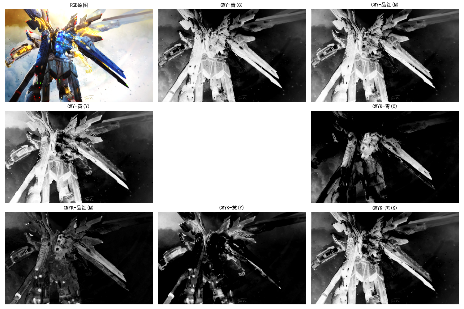
6.2.2 CMY 与 CMYK 颜色模型
CMY(青、品红、黄)是减色模型,通过吸收 RGB 光来生成颜色,适用于打印、印刷等反光设备;CMYK 在 CMY 基础上增加了黑色(K),解决 CMY 混合无法生成纯黑的问题。
实战代码:RGB 转 CMY/CMYK
import cv2
import numpy as np
import matplotlib.pyplot as plt

plt.rcParams['font.sans-serif'] = ['SimHei']
plt.rcParams['axes.unicode_minus'] = False

# RGB转CMY(归一化到0~1)
def rgb_to_cmy(rgb_img):
    # 将RGB值从0~255归一化到0~1
    rgb_normalized = rgb_img / 255.0
    # 计算CMY
    c = 1 - rgb_normalized[:, :, 0]
    m = 1 - rgb_normalized[:, :, 1]
    y = 1 - rgb_normalized[:, :, 2]
    return c, m, y

# RGB转CMYK
def rgb_to_cmyk(rgb_img):
    c, m, y = rgb_to_cmy(rgb_img)
    # 计算K值(黑色分量)
    k = np.min(np.stack([c, m, y], axis=-1), axis=-1)

    # 避免除以0
    k = np.where(k == 1, 0.9999, k)

    # 调整CMY分量
    c = (c - k) / (1 - k)
    m = (m - k) / (1 - k)
    y = (y - k) / (1 - k)

    return c, m, y, k

# 可视化CMY/CMYK结果
def cmyk_demo():
    # 读取图像并转换为RGB
    img = cv2.imread('test.jpg')
    img_rgb = cv2.cvtColor(img, cv2.COLOR_BGR2RGB)

    # 转换为CMY和CMYK
    c, m, y = rgb_to_cmy(img_rgb)
    c_k, m_k, y_k, k = rgb_to_cmyk(img_rgb)

    # 可视化
    plt.figure(figsize=(15, 10))

    # 原图
    plt.subplot(3, 4, 1)
    plt.imshow(img_rgb)
    plt.title('RGB原图')
    plt.axis('off')

    # CMY分量
    plt.subplot(3, 4, 2)
    plt.imshow(c, cmap='gray')
    plt.title('CMY-青(C)')
    plt.axis('off')

    plt.subplot(3, 4, 3)
    plt.imshow(m, cmap='gray')
    plt.title('CMY-品红(M)')
    plt.axis('off')

    plt.subplot(3, 4, 4)
    plt.imshow(y, cmap='gray')
    plt.title('CMY-黄(Y)')
    plt.axis('off')

    # CMYK分量
    plt.subplot(3, 4, 6)
    plt.imshow(c_k, cmap='gray')
    plt.title('CMYK-青(C)')
    plt.axis('off')

    plt.subplot(3, 4, 7)
    plt.imshow(m_k, cmap='gray')
    plt.title('CMYK-品红(M)')
    plt.axis('off')

    plt.subplot(3, 4, 8)
    plt.imshow(y_k, cmap='gray')
    plt.title('CMYK-黄(Y)')
    plt.axis('off')

    plt.subplot(3, 4, 9)
    plt.imshow(k, cmap='gray')
    plt.title('CMYK-黑(K)')
    plt.axis('off')

    plt.tight_layout()
    plt.show()

# 运行示例
if __name__ == '__main__':
    cmyk_demo()
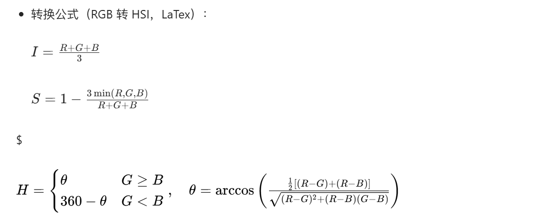
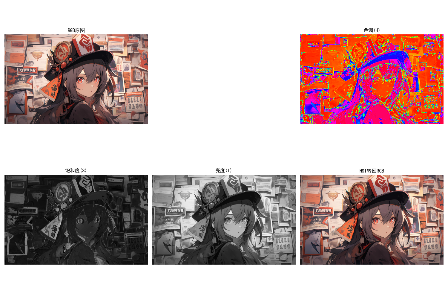
6.2.3 HSI 颜色模型
HSI(色调 H、饱和度 S、亮度 I)更符合人眼对颜色的感知,将颜色的亮度与色彩信息分离,非常适合彩色图像处理(如分割、增强)。
-
取值范围:
- H(色调):0~360°(或归一化到 0~1)
- S(饱和度):0~1
- I(亮度):0~1
实战代码:RGB转HSI及通道可视化
import cv2
import numpy as np
import matplotlib.pyplot as plt
import math

plt.rcParams['font.sans-serif'] = ['SimHei']
plt.rcParams['axes.unicode_minus'] = False

# RGB转HSI(输入RGB图像:0~255)
def rgb_to_hsi(rgb_img):
    # 归一化到0~1
    r = rgb_img[:, :, 0] / 255.0
    g = rgb_img[:, :, 1] / 255.0
    b = rgb_img[:, :, 2] / 255.0

    # 计算亮度I
    i = (r + g + b) / 3.0

    # 计算饱和度S
    min_rgb = np.min(np.stack([r, g, b], axis=-1), axis=-1)
    s = 1 - (3 / (r + g + b + 1e-6)) * min_rgb  # 加1e-6避免除以0

    # 计算色调H
    numerator = 0.5 * ((r - g) + (r - b))
    denominator = np.sqrt((r - g)**2 + (r - b) * (g - b)) + 1e-6
    theta = np.arccos(numerator / denominator)

    # 处理G < B的情况
    h = np.where(g >= b, theta, 2 * np.pi - theta)
    h = h / (2 * np.pi)  # 归一化到0~1

    # 处理灰度图像(S=0时H无意义,设为0)
    h = np.where(s == 0, 0, h)

    return h, s, i

# HSI转RGB(验证转换正确性)
def hsi_to_rgb(h, s, i):
    h = h * 2 * np.pi  # 转换为弧度
    r, g, b = np.zeros_like(h), np.zeros_like(h), np.zeros_like(h)

    # 分扇区计算
    # 扇区1: 0 <= h < 2π/3
    mask1 = (h >= 0) & (h < 2 * np.pi / 3)
    b[mask1] = i[mask1] * (1 - s[mask1])
    r[mask1] = i[mask1] * (1 + s[mask1] * np.cos(h[mask1]) / np.cos(np.pi/3 - h[mask1]))
    g[mask1] = 3 * i[mask1] - (r[mask1] + b[mask1])

    # 扇区2: 2π/3 <= h < 4π/3
    mask2 = (h >= 2 * np.pi / 3) & (h < 4 * np.pi / 3)
    h2 = h[mask2] - 2 * np.pi / 3
    r[mask2] = i[mask2] * (1 - s[mask2])
    g[mask2] = i[mask2] * (1 + s[mask2] * np.cos(h2) / np.cos(np.pi/3 - h2))
    b[mask2] = 3 * i[mask2] - (r[mask2] + g[mask2])

    # 扇区3: 4π/3 <= h < 2π
    mask3 = (h >= 4 * np.pi / 3) & (h < 2 * np.pi)
    h3 = h[mask3] - 4 * np.pi / 3
    g[mask3] = i[mask3] * (1 - s[mask3])
    b[mask3] = i[mask3] * (1 + s[mask3] * np.cos(h3) / np.cos(np.pi/3 - h3))
    r[mask3] = 3 * i[mask3] - (g[mask3] + b[mask3])

    # 归一化到0~255
    rgb = np.stack([r, g, b], axis=-1)
    rgb = np.clip(rgb, 0, 1) * 255
    rgb = rgb.astype(np.uint8)

    return rgb

# 可视化HSI通道
def hsi_demo():
    # 读取图像
    img = cv2.imread('test.jpg')
    img_rgb = cv2.cvtColor(img, cv2.COLOR_BGR2RGB)

    # RGB转HSI
    h, s, i = rgb_to_hsi(img_rgb)

    # HSI转回RGB(验证)
    img_rgb_back = hsi_to_rgb(h, s, i)

    # 可视化
    plt.figure(figsize=(15, 10))

    # 原图
    plt.subplot(2, 4, 1)
    plt.imshow(img_rgb)
    plt.title('RGB原图')
    plt.axis('off')

    # HSI各通道
    plt.subplot(2, 4, 2)
    plt.imshow(h, cmap='hsv')
    plt.title('色调(H)')
    plt.axis('off')

    plt.subplot(2, 4, 3)
    plt.imshow(s, cmap='gray')
    plt.title('饱和度(S)')
    plt.axis('off')

    plt.subplot(2, 4, 4)
    plt.imshow(i, cmap='gray')
    plt.title('亮度(I)')
    plt.axis('off')

    # 转回的RGB图
    plt.subplot(2, 4, 5)
    plt.imshow(img_rgb_back)
    plt.title('HSI转回RGB')
    plt.axis('off')

    plt.tight_layout()
    plt.show()

# 运行示例
if __name__ == '__main__':
    hsi_demo()
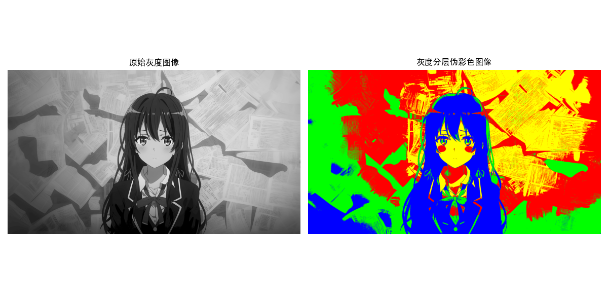
6.3 伪彩色图像处理
伪彩色处理是将灰度图像映射为彩色图像,增强人眼对灰度细节的识别能力,广泛应用于医学影像、遥感图像等领域。
6.3.1 灰度分层法
将灰度值划分为多个区间,每个区间赋予一种颜色,核心是“分层着色”。
实战代码:灰度分层伪彩色
import cv2
import numpy as np
import matplotlib.pyplot as plt

plt.rcParams['font.sans-serif'] = ['SimHei']
plt.rcParams['axes.unicode_minus'] = False

# 灰度分层法伪彩色
def gray_slicing_demo():
    # 读取灰度图像(若无灰度图,可将彩色图转灰度)
    gray_img = cv2.imread('test.jpg', 0)

    # 创建伪彩色图像
    pseudo_color = np.zeros((gray_img.shape[0], gray_img.shape[1], 3), dtype=np.uint8)

    # 定义灰度分层区间和对应颜色
    # 区间1: 0~63 → 蓝色
    mask1 = (gray_img >= 0) & (gray_img < 64)
    pseudo_color[mask1] = [0, 0, 255]

    # 区间2: 64~127 → 绿色
    mask2 = (gray_img >= 64) & (gray_img < 128)
    pseudo_color[mask2] = [0, 255, 0]

    # 区间3: 128~191 → 红色
    mask3 = (gray_img >= 128) & (gray_img < 192)
    pseudo_color[mask3] = [255, 0, 0]

    # 区间4: 192~255 → 黄色
    mask4 = (gray_img >= 192) & (gray_img <= 255)
    pseudo_color[mask4] = [255, 255, 0]

    # 可视化对比
    plt.figure(figsize=(12, 6))

    plt.subplot(1, 2, 1)
    plt.imshow(gray_img, cmap='gray')
    plt.title('原始灰度图像')
    plt.axis('off')

    plt.subplot(1, 2, 2)
    plt.imshow(pseudo_color)
    plt.title('灰度分层伪彩色图像')
    plt.axis('off')

    plt.tight_layout()
    plt.show()

# 运行示例
if __name__ == '__main__':
    gray_slicing_demo()
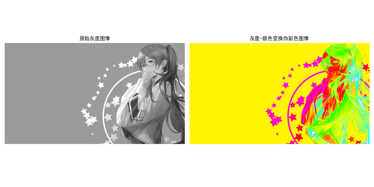
6.3.2 灰度-颜色变换法
将灰度值通过数学变换映射到RGB三个通道,生成连续的伪彩色效果,比灰度分层法更平滑。
实战代码:灰度-颜色变换伪彩色
import cv2
import numpy as np
import matplotlib.pyplot as plt

plt.rcParams['font.sans-serif'] = ['SimHei']
plt.rcParams['axes.unicode_minus'] = False

# 灰度-颜色变换法伪彩色(彩虹色映射)
def gray_color_transform_demo():
    # 读取灰度图像
    gray_img = cv2.imread('test.jpg', 0)
    h, w = gray_img.shape

    # 归一化灰度值到0~1
    gray_normalized = gray_img / 255.0

    # 定义RGB变换函数(彩虹色:黑→蓝→青→绿→黄→红→白)
    r = np.zeros_like(gray_normalized)
    g = np.zeros_like(gray_normalized)
    b = np.zeros_like(gray_normalized)

    # 蓝区(0~0.2)
    mask1 = gray_normalized <= 0.2
    b[mask1] = 1.0
    r[mask1] = gray_normalized[mask1] / 0.2
    g[mask1] = gray_normalized[mask1] / 0.2

    # 青区(0.2~0.4)
    mask2 = (gray_normalized > 0.2) & (gray_normalized <= 0.4)
    b[mask2] = 1.0 - (gray_normalized[mask2] - 0.2) / 0.2
    g[mask2] = 1.0
    r[mask2] = (gray_normalized[mask2] - 0.2) / 0.2

    # 绿区(0.4~0.6)
    mask3 = (gray_normalized > 0.4) & (gray_normalized <= 0.6)
    b[mask3] = 0.0
    g[mask3] = 1.0
    r[mask3] = 1.0 - (gray_normalized[mask3] - 0.4) / 0.2

    # 黄区(0.6~0.8)
    mask4 = (gray_normalized > 0.6) & (gray_normalized <= 0.8)
    b[mask4] = 0.0
    g[mask4] = 1.0 - (gray_normalized[mask4] - 0.6) / 0.2
    r[mask4] = 1.0

    # 红区(0.8~1.0)
    mask5 = gray_normalized > 0.8
    b[mask5] = (gray_normalized[mask5] - 0.8) / 0.2
    g[mask5] = 0.0
    r[mask5] = 1.0

    # 组合RGB图像
    pseudo_color = np.stack([r, g, b], axis=-1)
    pseudo_color = (pseudo_color * 255).astype(np.uint8)

    # 可视化对比
    plt.figure(figsize=(12, 6))

    plt.subplot(1, 2, 1)
    plt.imshow(gray_img, cmap='gray')
    plt.title('原始灰度图像')
    plt.axis('off')

    plt.subplot(1, 2, 2)
    plt.imshow(pseudo_color)
    plt.title('灰度-颜色变换伪彩色图像')
    plt.axis('off')

    plt.tight_layout()
    plt.show()

# 运行示例
if __name__ == '__main__':
    gray_color_transform_demo()
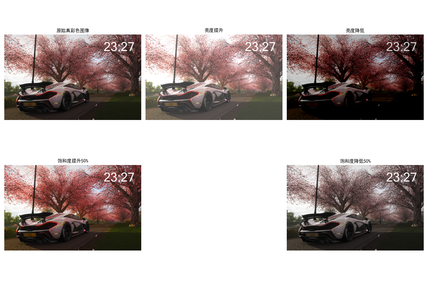
6.4 真彩色图像处理基础
真彩色图像是指每个像素由RGB(或其他颜色模型)三个通道组成,能真实还原场景颜色的图像。
核心处理原则
- 可对RGB三个通道分别处理后再合并;
- 可转换到HSI空间,对亮度/饱和度/色调单独处理(更符合人眼感知);
- 处理时需保持通道间的一致性,避免颜色失真。
实战代码:真彩色图像基本操作
import cv2
import numpy as np
import matplotlib.pyplot as plt

plt.rcParams['font.sans-serif'] = ['SimHei']
plt.rcParams['axes.unicode_minus'] = False

# 真彩色图像基础操作
def true_color_basic_ops():
    # 读取真彩色图像
    img = cv2.imread('test.jpg')
    img_rgb = cv2.cvtColor(img, cv2.COLOR_BGR2RGB)

    # 1. 亮度调整(RGB通道整体加减)
    img_bright = cv2.add(img_rgb, np.ones_like(img_rgb) * 50)  # 增亮
    img_dark = cv2.subtract(img_rgb, np.ones_like(img_rgb) * 50)  # 调暗
    img_bright = np.clip(img_bright, 0, 255).astype(np.uint8)
    img_dark = np.clip(img_dark, 0, 255).astype(np.uint8)

    # 2. 饱和度调整(HSI空间)
    h, s, i = rgb_to_hsi(img_rgb)
    s_enhance = s * 1.5  # 饱和度提升50%
    s_reduce = s * 0.5   # 饱和度降低50%
    s_enhance = np.clip(s_enhance, 0, 1)
    s_reduce = np.clip(s_reduce, 0, 1)
    img_s_enhance = hsi_to_rgb(h, s_enhance, i)
    img_s_reduce = hsi_to_rgb(h, s_reduce, i)

    # 可视化
    plt.figure(figsize=(15, 10))

    plt.subplot(2, 3, 1)
    plt.imshow(img_rgb)
    plt.title('原始真彩色图像')
    plt.axis('off')

    plt.subplot(2, 3, 2)
    plt.imshow(img_bright)
    plt.title('亮度提升')
    plt.axis('off')

    plt.subplot(2, 3, 3)
    plt.imshow(img_dark)
    plt.title('亮度降低')
    plt.axis('off')

    plt.subplot(2, 3, 4)
    plt.imshow(img_s_enhance)
    plt.title('饱和度提升50%')
    plt.axis('off')

    plt.subplot(2, 3, 5)
    plt.imshow(img_s_reduce)
    plt.title('饱和度降低50%')
    plt.axis('off')

    plt.tight_layout()
    plt.show()

# 复用之前定义的rgb_to_hsi和hsi_to_rgb函数
def rgb_to_hsi(rgb_img):
    r = rgb_img[:, :, 0] / 255.0
    g = rgb_img[:, :, 1] / 255.0
    b = rgb_img[:, :, 2] / 255.0
    i = (r + g + b) / 3.0
    min_rgb = np.min(np.stack([r, g, b], axis=-1), axis=-1)
    s = 1 - (3 / (r + g + b + 1e-6)) * min_rgb
    numerator = 0.5 * ((r - g) + (r - b))
    denominator = np.sqrt((r - g)**2 + (r - b) * (g - b)) + 1e-6
    theta = np.arccos(numerator / denominator)
    h = np.where(g >= b, theta, 2 * np.pi - theta)
    h = h / (2 * np.pi)
    h = np.where(s == 0, 0, h)
    return h, s, i

def hsi_to_rgb(h, s, i):
    h = h * 2 * np.pi
    r, g, b = np.zeros_like(h), np.zeros_like(h), np.zeros_like(h)
    mask1 = (h >= 0) & (h < 2 * np.pi / 3)
    b[mask1] = i[mask1] * (1 - s[mask1])
    r[mask1] = i[mask1] * (1 + s[mask1] * np.cos(h[mask1]) / np.cos(np.pi/3 - h[mask1]))
    g[mask1] = 3 * i[mask1] - (r[mask1] + b[mask1])
    mask2 = (h >= 2 * np.pi / 3) & (h < 4 * np.pi / 3)
    h2 = h[mask2] - 2 * np.pi / 3
    r[mask2] = i[mask2] * (1 - s[mask2])
    g[mask2] = i[mask2] * (1 + s[mask2] * np.cos(h2) / np.cos(np.pi/3 - h2))
    b[mask2] = 3 * i[mask2] - (r[mask2] + g[mask2])
    mask3 = (h >= 4 * np.pi / 3) & (h < 2 * np.pi)
    h3 = h[mask3] - 4 * np.pi / 3
    g[mask3] = i[mask3] * (1 - s[mask3])
    b[mask3] = i[mask3] * (1 + s[mask3] * np.cos(h3) / np.cos(np.pi/3 - h3))
    r[mask3] = 3 * i[mask3] - (g[mask3] + b[mask3])
    rgb = np.stack([r, g, b], axis=-1)
    rgb = np.clip(rgb, 0, 1) * 255
    rgb = rgb.astype(np.uint8)
    return rgb

# 运行示例
if __name__ == '__main__':
    true_color_basic_ops()
6.5 彩色变换
彩色变换是对彩色图像的像素值进行数学变换,实现颜色调整、增强等效果。
6.5.1 变换模型构建
彩色变换的通用模型为:Cout=T(Cin),其中Cin是输入颜色向量,Cout是输出颜色向量,T是变换函数(线性/非线性)。
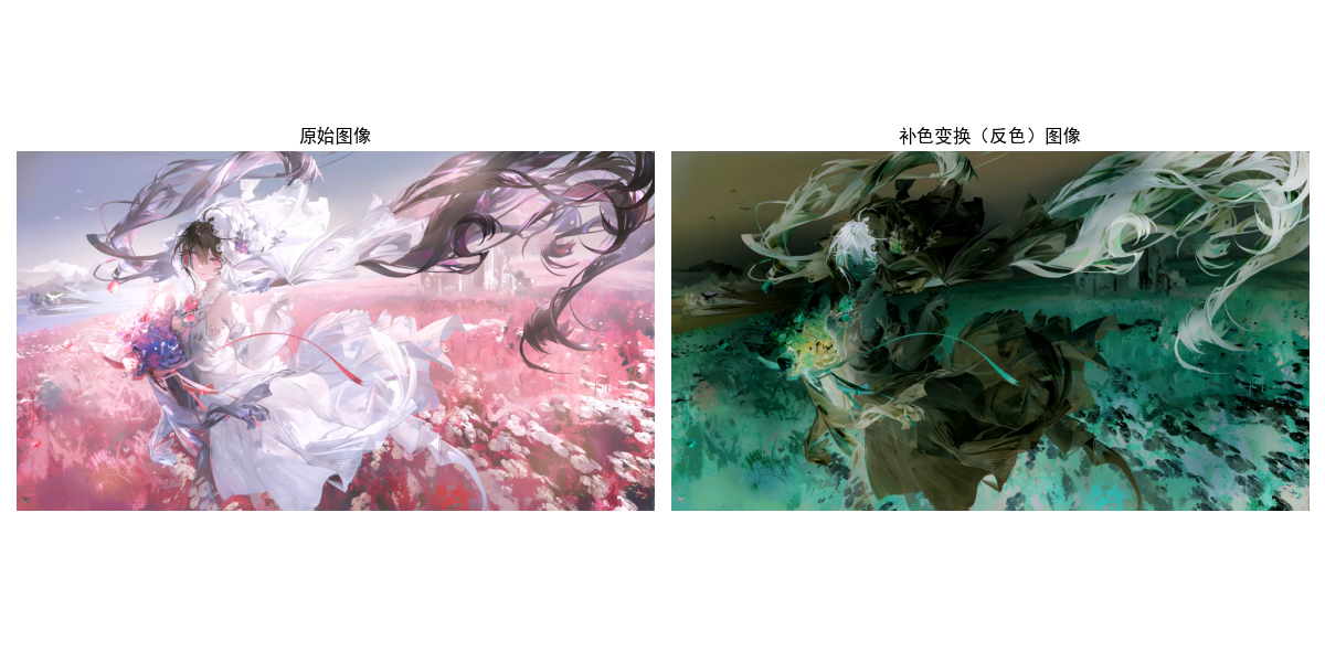
6.5.2 补色变换
补色是指两种颜色混合后生成白色(RGB)或黑色(CMY),补色变换可实现“反色”效果。
实战代码:补色变换
import cv2
import numpy as np
import matplotlib.pyplot as plt

plt.rcParams['font.sans-serif'] = ['SimHei']
plt.rcParams['axes.unicode_minus'] = False

# 补色变换(反色)
def complementary_color_demo():
    # 读取图像
    img = cv2.imread('test.jpg')
    img_rgb = cv2.cvtColor(img, cv2.COLOR_BGR2RGB)

    # 补色变换:255 - 原像素值
    complementary_img = 255 - img_rgb

    # 可视化对比
    plt.figure(figsize=(12, 6))

    plt.subplot(1, 2, 1)
    plt.imshow(img_rgb)
    plt.title('原始图像')
    plt.axis('off')

    plt.subplot(1, 2, 2)
    plt.imshow(complementary_img)
    plt.title('补色变换(反色)图像')
    plt.axis('off')

    plt.tight_layout()
    plt.show()

# 运行示例
if __name__ == '__main__':
    complementary_color_demo()
6.5.3 彩色分层
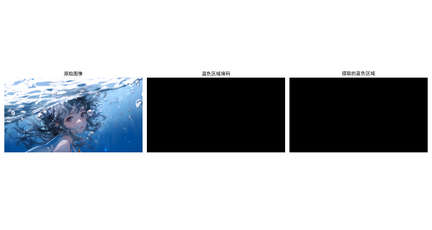
将彩色图像按颜色通道或颜色区间分层提取,用于目标识别、特征提取。
实战代码:彩色分层提取红色区域
import cv2
import numpy as np
import matplotlib.pyplot as plt

plt.rcParams['font.sans-serif'] = ['SimHei']
plt.rcParams['axes.unicode_minus'] = False

# 彩色分层提取红色区域
def color_slicing_demo():
    # 读取图像
    img = cv2.imread('test.jpg')
    img_rgb = cv2.cvtColor(img, cv2.COLOR_BGR2RGB)

    # 定义红色区间(RGB)
    lower_red = np.array([150, 0, 0])
    upper_red = np.array([255, 100, 100])

    # 生成掩码(提取红色区域)
    mask = cv2.inRange(img_rgb, lower_red, upper_red)
    red_region = cv2.bitwise_and(img_rgb, img_rgb, mask=mask)

    # 可视化
    plt.figure(figsize=(15, 5))

    plt.subplot(1, 3, 1)
    plt.imshow(img_rgb)
    plt.title('原始图像')
    plt.axis('off')

    plt.subplot(1, 3, 2)
    plt.imshow(mask, cmap='gray')
    plt.title('红色区域掩码')
    plt.axis('off')

    plt.subplot(1, 3, 3)
    plt.imshow(red_region)
    plt.title('提取的红色区域')
    plt.axis('off')

    plt.tight_layout()
    plt.show()

# 运行示例
if __name__ == '__main__':
    color_slicing_demo()

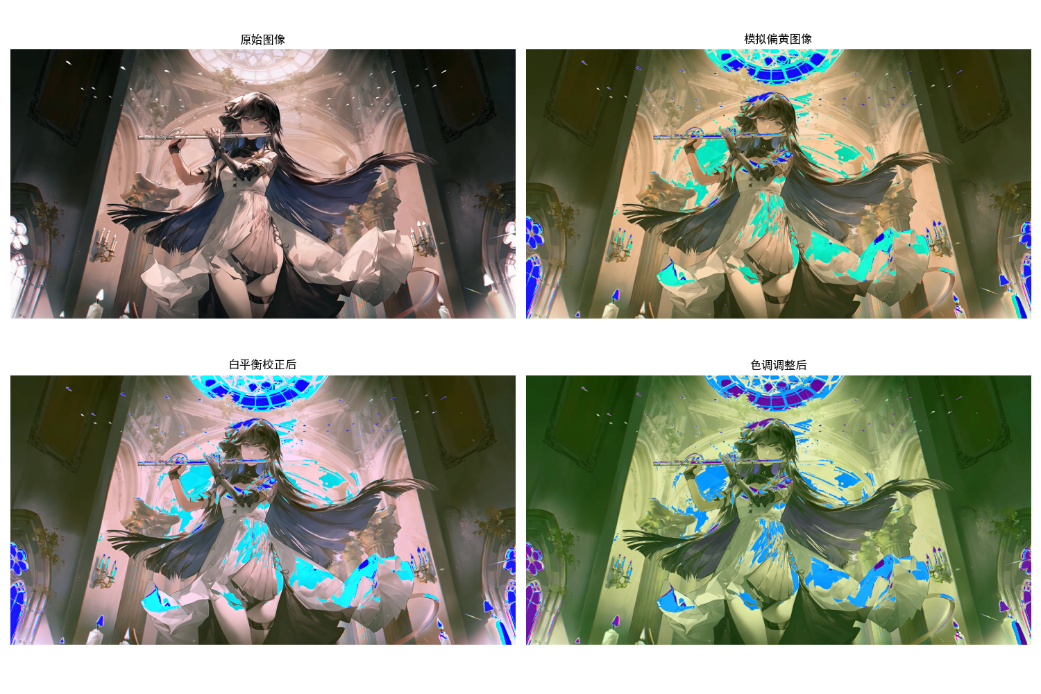
6.5.4 色调与色彩校正
通过调整HSI空间的色调或RGB通道的增益,校正图像的偏色问题。
实战代码:色调调整与白平衡校正
import cv2
import numpy as np
import matplotlib.pyplot as plt

plt.rcParams['font.sans-serif'] = ['SimHei']
plt.rcParams['axes.unicode_minus'] = False

# 色调调整与白平衡校正
def color_correction_demo():
    # 读取图像(模拟偏色图像)
    img = cv2.imread('test.jpg')
    img_rgb = cv2.cvtColor(img, cv2.COLOR_BGR2RGB)

    # 1. 模拟偏黄(增加红、绿通道值)
    yellow_cast = img_rgb.copy()
    yellow_cast[:, :, 0] = np.clip(yellow_cast[:, :, 0] + 30, 0, 255)
    yellow_cast[:, :, 1] = np.clip(yellow_cast[:, :, 1] + 30, 0, 255)

    # 2. 白平衡校正(灰度世界法)
    # 计算各通道均值
    r_mean = np.mean(yellow_cast[:, :, 0])
    g_mean = np.mean(yellow_cast[:, :, 1])
    b_mean = np.mean(yellow_cast[:, :, 2])
    # 计算增益
    gain_r = g_mean / r_mean
    gain_b = g_mean / b_mean
    # 校正
    white_balance = yellow_cast.copy().astype(np.float32)
    white_balance[:, :, 0] *= gain_r
    white_balance[:, :, 2] *= gain_b
    white_balance = np.clip(white_balance, 0, 255).astype(np.uint8)

    # 3. 色调调整(HSI空间)
    h, s, i = rgb_to_hsi(yellow_cast)
    h_shift = (h + 0.1) % 1.0  # 色调偏移10%
    hsi_adjust = hsi_to_rgb(h_shift, s, i)

    # 可视化
    plt.figure(figsize=(15, 10))

    plt.subplot(2, 2, 1)
    plt.imshow(img_rgb)
    plt.title('原始图像')
    plt.axis('off')

    plt.subplot(2, 2, 2)
    plt.imshow(yellow_cast)
    plt.title('模拟偏黄图像')
    plt.axis('off')

    plt.subplot(2, 2, 3)
    plt.imshow(white_balance)
    plt.title('白平衡校正后')
    plt.axis('off')

    plt.subplot(2, 2, 4)
    plt.imshow(hsi_adjust)
    plt.title('色调调整后')
    plt.axis('off')

    plt.tight_layout()
    plt.show()

# 复用rgb_to_hsi和hsi_to_rgb函数
def rgb_to_hsi(rgb_img):
    r = rgb_img[:, :, 0] / 255.0
    g = rgb_img[:, :, 1] / 255.0
    b = rgb_img[:, :, 2] / 255.0
    i = (r + g + b) / 3.0
    min_rgb = np.min(np.stack([r, g, b], axis=-1), axis=-1)
    s = 1 - (3 / (r + g + b + 1e-6)) * min_rgb
    numerator = 0.5 * ((r - g) + (r - b))
    denominator = np.sqrt((r - g)**2 + (r - b) * (g - b)) + 1e-6
    theta = np.arccos(numerator / denominator)
    h = np.where(g >= b, theta, 2 * np.pi - theta)
    h = h / (2 * np.pi)
    h = np.where(s == 0, 0, h)
    return h, s, i

def hsi_to_rgb(h, s, i):
    h = h * 2 * np.pi
    r, g, b = np.zeros_like(h), np.zeros_like(h), np.zeros_like(h)
    mask1 = (h >= 0) & (h < 2 * np.pi / 3)
    b[mask1] = i[mask1] * (1 - s[mask1])
    r[mask1] = i[mask1] * (1 + s[mask1] * np.cos(h[mask1]) / np.cos(np.pi/3 - h[mask1]))
    g[mask1] = 3 * i[mask1] - (r[mask1] + b[mask1])
    mask2 = (h >= 2 * np.pi / 3) & (h < 4 * np.pi / 3)
    h2 = h[mask2] - 2 * np.pi / 3
    r[mask2] = i[mask2] * (1 - s[mask2])
    g[mask2] = i[mask2] * (1 + s[mask2] * np.cos(h2) / np.cos(np.pi/3 - h2))
    b[mask2] = 3 * i[mask2] - (r[mask2] + g[mask2])
    mask3 = (h >= 4 * np.pi / 3) & (h < 2 * np.pi)
    h3 = h[mask3] - 4 * np.pi / 3
    g[mask3] = i[mask3] * (1 - s[mask3])
    b[mask3] = i[mask3] * (1 + s[mask3] * np.cos(h3) / np.cos(np.pi/3 - h3))
    r[mask3] = 3 * i[mask3] - (g[mask3] + b[mask3])
    rgb = np.stack([r, g, b], axis=-1)
    rgb = np.clip(rgb, 0, 1) * 255
    rgb = rgb.astype(np.uint8)
    return rgb

# 运行示例
if __name__ == '__main__':
    color_correction_demo()
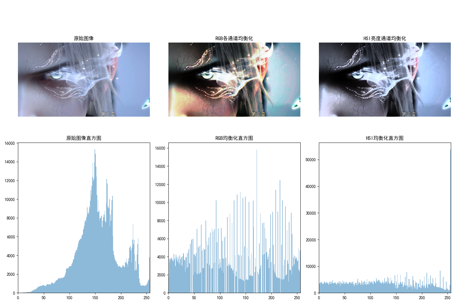
6.5.5 直方图处理
对彩色图像的各通道分别进行直方图均衡化,增强对比度。
实战代码:彩色图像直方图均衡化
import cv2
import numpy as np
import matplotlib.pyplot as plt

plt.rcParams['font.sans-serif'] = ['SimHei']
plt.rcParams['axes.unicode_minus'] = False

# 彩色图像直方图均衡化
def color_hist_equalization_demo():
    # 读取图像
    img = cv2.imread('test.jpg')
    img_rgb = cv2.cvtColor(img, cv2.COLOR_BGR2RGB)

    # 方法1:RGB各通道分别均衡化
    r, g, b = cv2.split(img_rgb)
    r_eq = cv2.equalizeHist(r)
    g_eq = cv2.equalizeHist(g)
    b_eq = cv2.equalizeHist(b)
    rgb_eq = cv2.merge([r_eq, g_eq, b_eq])

    # 方法2:HSI空间亮度通道均衡化(更自然)
    h, s, i = rgb_to_hsi(img_rgb)
    i_eq = cv2.equalizeHist((i * 255).astype(np.uint8)) / 255.0
    hsi_eq = hsi_to_rgb(h, s, i_eq)

    # 可视化对比
    plt.figure(figsize=(15, 10))

    plt.subplot(2, 3, 1)
    plt.imshow(img_rgb)
    plt.title('原始图像')
    plt.axis('off')

    plt.subplot(2, 3, 2)
    plt.imshow(rgb_eq)
    plt.title('RGB各通道均衡化')
    plt.axis('off')

    plt.subplot(2, 3, 3)
    plt.imshow(hsi_eq)
    plt.title('HSI亮度通道均衡化')
    plt.axis('off')

    # 绘制直方图
    plt.subplot(2, 3, 4)
    plt.hist(img_rgb.ravel(), 256, [0, 256], alpha=0.5)
    plt.title('原始图像直方图')
    plt.xlim([0, 256])

    plt.subplot(2, 3, 5)
    plt.hist(rgb_eq.ravel(), 256, [0, 256], alpha=0.5)
    plt.title('RGB均衡化直方图')
    plt.xlim([0, 256])

    plt.subplot(2, 3, 6)
    plt.hist(hsi_eq.ravel(), 256, [0, 256], alpha=0.5)
    plt.title('HSI均衡化直方图')
    plt.xlim([0, 256])

    plt.tight_layout()
    plt.show()

# 复用rgb_to_hsi和hsi_to_rgb函数
def rgb_to_hsi(rgb_img):
    r = rgb_img[:, :, 0] / 255.0
    g = rgb_img[:, :, 1] / 255.0
    b = rgb_img[:, :, 2] / 255.0
    i = (r + g + b) / 3.0
    min_rgb = np.min(np.stack([r, g, b], axis=-1), axis=-1)
    s = 1 - (3 / (r + g + b + 1e-6)) * min_rgb
    numerator = 0.5 * ((r - g) + (r - b))
    denominator = np.sqrt((r - g)**2 + (r - b) * (g - b)) + 1e-6
    theta = np.arccos(numerator / denominator)
    h = np.where(g >= b, theta, 2 * np.pi - theta)
    h = h / (2 * np.pi)
    h = np.where(s == 0, 0, h)
    return h, s, i

def hsi_to_rgb(h, s, i):
    h = h * 2 * np.pi
    r, g, b = np.zeros_like(h), np.zeros_like(h), np.zeros_like(h)
    mask1 = (h >= 0) & (h < 2 * np.pi / 3)
    b[mask1] = i[mask1] * (1 - s[mask1])
    r[mask1] = i[mask1] * (1 + s[mask1] * np.cos(h[mask1]) / np.cos(np.pi/3 - h[mask1]))
    g[mask1] = 3 * i[mask1] - (r[mask1] + b[mask1])
    mask2 = (h >= 2 * np.pi / 3) & (h < 4 * np.pi / 3)
    h2 = h[mask2] - 2 * np.pi / 3
    r[mask2] = i[mask2] * (1 - s[mask2])
    g[mask2] = i[mask2] * (1 + s[mask2] * np.cos(h2) / np.cos(np.pi/3 - h2))
    b[mask2] = 3 * i[mask2] - (r[mask2] + g[mask2])
    mask3 = (h >= 4 * np.pi / 3) & (h < 2 * np.pi)
    h3 = h[mask3] - 4 * np.pi / 3
    g[mask3] = i[mask3] * (1 - s[mask3])
    b[mask3] = i[mask3] * (1 + s[mask3] * np.cos(h3) / np.cos(np.pi/3 - h3))
    r[mask3] = 3 * i[mask3] - (g[mask3] + b[mask3])
    rgb = np.stack([r, g, b], axis=-1)
    rgb = np.clip(rgb, 0, 1) * 255
    rgb = rgb.astype(np.uint8)
    return rgb

# 运行示例
if __name__ == '__main__':
    color_hist_equalization_demo()
6.6 彩色图像的平滑与锐化
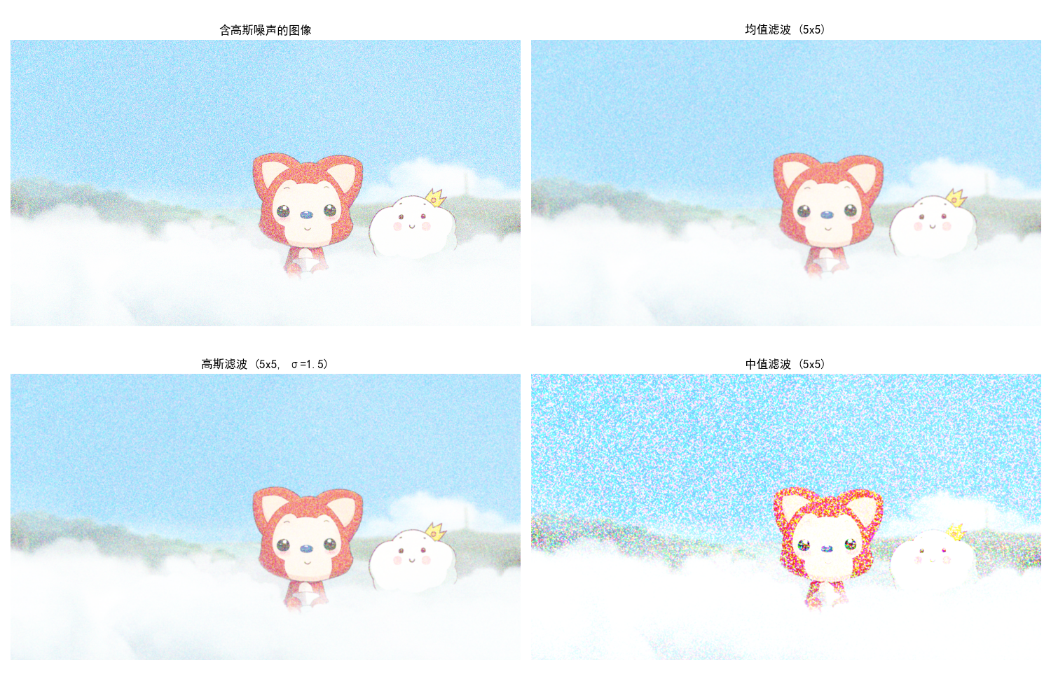
6.6.1 彩色图像平滑
对彩色图像进行滤波去噪,可对RGB各通道分别滤波,或在HSI空间对亮度通道滤波。
实战代码:彩色图像平滑
import cv2
import numpy as np
import matplotlib.pyplot as plt

plt.rcParams['font.sans-serif'] = ['SimHei']
plt.rcParams['axes.unicode_minus'] = False

# 彩色图像平滑
def color_smoothing_demo():
    # 读取图像并添加噪声
    img = cv2.imread('test.jpg')
    img_rgb = cv2.cvtColor(img, cv2.COLOR_BGR2RGB)

    # 添加高斯噪声
    noise = np.random.normal(0, 20, img_rgb.shape).astype(np.uint8)
    noisy_img = cv2.add(img_rgb, noise)
    noisy_img = np.clip(noisy_img, 0, 255).astype(np.uint8)

    # 1. 均值滤波
    mean_filter = cv2.blur(noisy_img, (5, 5))

    # 2. 高斯滤波
    gaussian_filter = cv2.GaussianBlur(noisy_img, (5, 5), 1.5)

    # 3. 中值滤波(去椒盐噪声效果好)
    median_filter = cv2.medianBlur(noisy_img, 5)

    # 可视化对比
    plt.figure(figsize=(15, 10))

    plt.subplot(2, 2, 1)
    plt.imshow(noisy_img)
    plt.title('含高斯噪声的图像')
    plt.axis('off')

    plt.subplot(2, 2, 2)
    plt.imshow(mean_filter)
    plt.title('均值滤波 (5x5)')
    plt.axis('off')

    plt.subplot(2, 2, 3)
    plt.imshow(gaussian_filter)
    plt.title('高斯滤波 (5x5, σ=1.5)')
    plt.axis('off')

    plt.subplot(2, 2, 4)
    plt.imshow(median_filter)
    plt.title('中值滤波 (5x5)')
    plt.axis('off')

    plt.tight_layout()
    plt.show()

# 运行示例
if __name__ == '__main__':
    color_smoothing_demo()
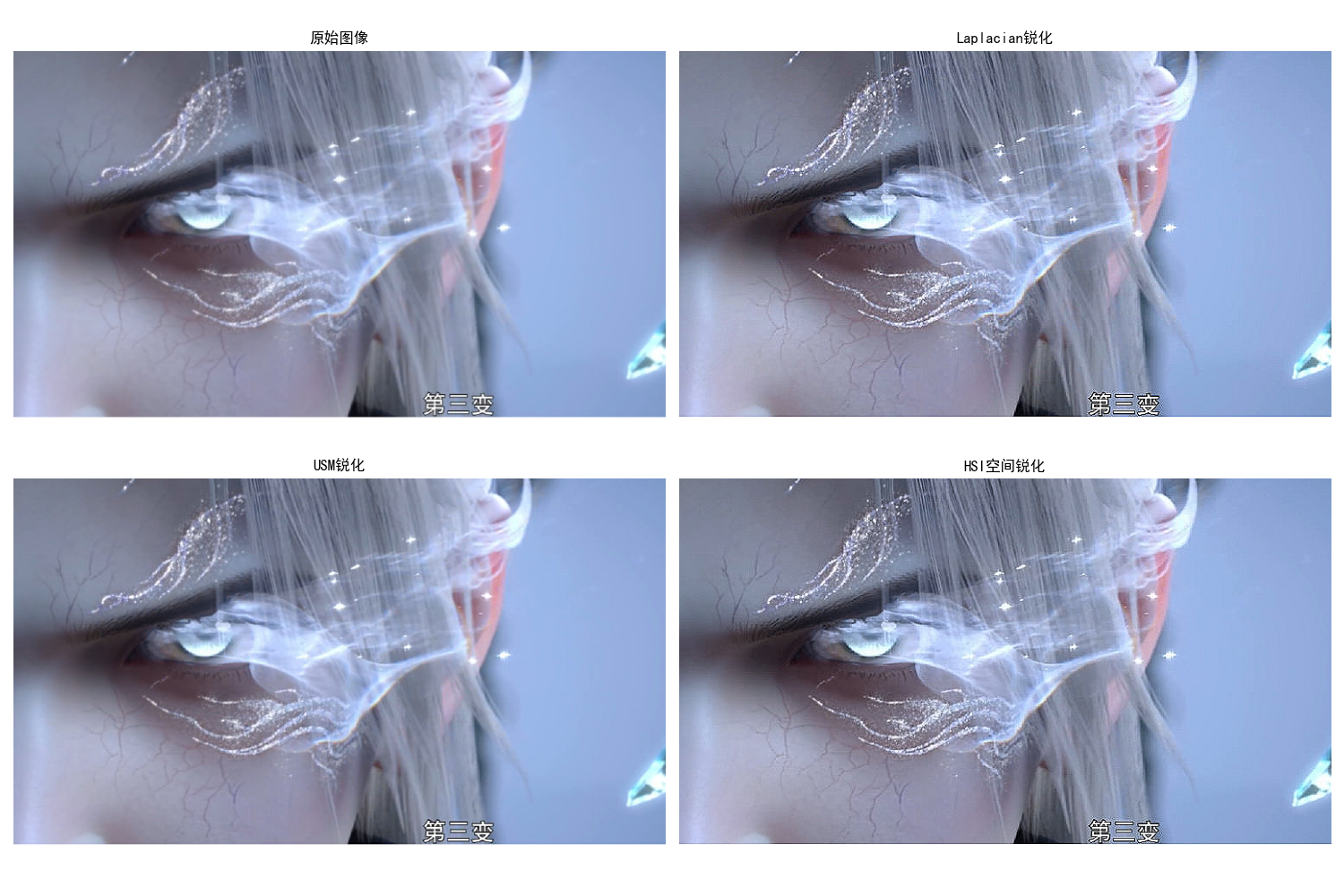
6.6.2 彩色图像锐化
通过增强图像的边缘和细节,提升图像的清晰度。
实战代码:彩色图像锐化
import cv2
import numpy as np
import matplotlib.pyplot as plt

plt.rcParams['font.sans-serif'] = ['SimHei']
plt.rcParams['axes.unicode_minus'] = False

# 彩色图像锐化
def color_sharpening_demo():
    # 读取图像
    img = cv2.imread('test.jpg')
    img_rgb = cv2.cvtColor(img, cv2.COLOR_BGR2RGB)

    # 1. Laplacian锐化
    laplacian_kernel = np.array([[0, -1, 0], [-1, 5, -1], [0, -1, 0]])
    laplacian_sharpen = cv2.filter2D(img_rgb, -1, laplacian_kernel)

    # 2. USM锐化(非锐化掩模)
    blur = cv2.GaussianBlur(img_rgb, (5, 5), 2)
    usm_sharpen = cv2.addWeighted(img_rgb, 1.5, blur, -0.5, 0)

    # 3. HSI空间锐化(仅锐化亮度通道)
    h, s, i = rgb_to_hsi(img_rgb)
    i_sharpen = cv2.filter2D((i * 255).astype(np.uint8), -1, laplacian_kernel) / 255.0
    i_sharpen = np.clip(i_sharpen, 0, 1)
    hsi_sharpen = hsi_to_rgb(h, s, i_sharpen)

    # 可视化对比
    plt.figure(figsize=(15, 10))

    plt.subplot(2, 2, 1)
    plt.imshow(img_rgb)
    plt.title('原始图像')
    plt.axis('off')

    plt.subplot(2, 2, 2)
    plt.imshow(laplacian_sharpen)
    plt.title('Laplacian锐化')
    plt.axis('off')

    plt.subplot(2, 2, 3)
    plt.imshow(usm_sharpen)
    plt.title('USM锐化')
    plt.axis('off')

    plt.subplot(2, 2, 4)
    plt.imshow(hsi_sharpen)
    plt.title('HSI空间锐化')
    plt.axis('off')

    plt.tight_layout()
    plt.show()

# 复用rgb_to_hsi和hsi_to_rgb函数
def rgb_to_hsi(rgb_img):
    r = rgb_img[:, :, 0] / 255.0
    g = rgb_img[:, :, 1] / 255.0
    b = rgb_img[:, :, 2] / 255.0
    i = (r + g + b) / 3.0
    min_rgb = np.min(np.stack([r, g, b], axis=-1), axis=-1)
    s = 1 - (3 / (r + g + b + 1e-6)) * min_rgb
    numerator = 0.5 * ((r - g) + (r - b))
    denominator = np.sqrt((r - g)**2 + (r - b) * (g - b)) + 1e-6
    theta = np.arccos(numerator / denominator)
    h = np.where(g >= b, theta, 2 * np.pi - theta)
    h = h / (2 * np.pi)
    h = np.where(s == 0, 0, h)
    return h, s, i

def hsi_to_rgb(h, s, i):
    h = h * 2 * np.pi
    r, g, b = np.zeros_like(h), np.zeros_like(h), np.zeros_like(h)
    mask1 = (h >= 0) & (h < 2 * np.pi / 3)
    b[mask1] = i[mask1] * (1 - s[mask1])
    r[mask1] = i[mask1] * (1 + s[mask1] * np.cos(h[mask1]) / np.cos(np.pi/3 - h[mask1]))
    g[mask1] = 3 * i[mask1] - (r[mask1] + b[mask1])
    mask2 = (h >= 2 * np.pi / 3) & (h < 4 * np.pi / 3)
    h2 = h[mask2] - 2 * np.pi / 3
    r[mask2] = i[mask2] * (1 - s[mask2])
    g[mask2] = i[mask2] * (1 + s[mask2] * np.cos(h2) / np.cos(np.pi/3 - h2))
    b[mask2] = 3 * i[mask2] - (r[mask2] + g[mask2])
    mask3 = (h >= 4 * np.pi / 3) & (h < 2 * np.pi)
    h3 = h[mask3] - 4 * np.pi / 3
    g[mask3] = i[mask3] * (1 - s[mask3])
    b[mask3] = i[mask3] * (1 + s[mask3] * np.cos(h3) / np.cos(np.pi/3 - h3))
    r[mask3] = 3 * i[mask3] - (g[mask3] + b[mask3])
    rgb = np.stack([r, g, b], axis=-1)
    rgb = np.clip(rgb, 0, 1) * 255
    rgb = rgb.astype(np.uint8)
    return rgb

# 运行示例
if __name__ == '__main__':
    color_sharpening_demo()
6.7 基于色彩的图像分割
基于颜色特征将图像划分为不同的区域,是目标检测、图像分析的基础。
6.7.1 HSI 颜色空间中的分割
HSI空间分离了亮度和色彩信息,分割效果更稳定(不受光照影响)。
实战代码:HSI空间颜色分割
import cv2
import numpy as np
import matplotlib.pyplot as plt

plt.rcParams['font.sans-serif'] = ['SimHei']
plt.rcParams['axes.unicode_minus'] = False

# HSI空间颜色分割(提取绿色区域)
def hsi_segmentation_demo():
    # 读取图像
    img = cv2.imread('test.jpg')
    img_rgb = cv2.cvtColor(img, cv2.COLOR_BGR2RGB)

    # 转换到HSI空间
    h, s, i = rgb_to_hsi(img_rgb)

    # 定义绿色的HSI范围
    # 色调H:0.2~0.4(对应60°~120°),饱和度S:>0.2,亮度I:>0.1
    h_mask = (h >= 0.2) & (h <= 0.4)
    s_mask = (s >= 0.2)
    i_mask = (i >= 0.1)
    green_mask = h_mask & s_mask & i_mask

    # 提取绿色区域
    green_region = np.zeros_like(img_rgb)
    green_region[green_mask] = img_rgb[green_mask]

    # 可视化
    plt.figure(figsize=(15, 5))

    plt.subplot(1, 3, 1)
    plt.imshow(img_rgb)
    plt.title('原始图像')
    plt.axis('off')

    plt.subplot(1, 3, 2)
    plt.imshow(green_mask.astype(np.uint8) * 255, cmap='gray')
    plt.title('绿色区域掩码')
    plt.axis('off')

    plt.subplot(1, 3, 3)
    plt.imshow(green_region)
    plt.title('提取的绿色区域')
    plt.axis('off')

    plt.tight_layout()
    plt.show()

# 复用rgb_to_hsi函数
def rgb_to_hsi(rgb_img):
    r = rgb_img[:, :, 0] / 255.0
    g = rgb_img[:, :, 1] / 255.0
    b = rgb_img[:, :, 2] / 255.0
    i = (r + g + b) / 3.0
    min_rgb = np.min(np.stack([r, g, b], axis=-1), axis=-1)
    s = 1 - (3 / (r + g + b + 1e-6)) * min_rgb
    numerator = 0.5 * ((r - g) + (r - b))
    denominator = np.sqrt((r - g)**2 + (r - b) * (g - b)) + 1e-6
    theta = np.arccos(numerator / denominator)
    h = np.where(g >= b, theta, 2 * np.pi - theta)
    h = h / (2 * np.pi)
    h = np.where(s == 0, 0, h)
    return h, s, i

# 运行示例
if __name__ == '__main__':
    hsi_segmentation_demo()
6.7.2 RGB 向量空间中的分割
将每个像素视为RGB三维向量,通过距离度量(如欧氏距离)分割目标颜色。
实战代码:RGB向量空间分割
import cv2
import numpy as np
import matplotlib.pyplot as plt

plt.rcParams['font.sans-serif'] = ['SimHei']
plt.rcParams['axes.unicode_minus'] = False

# RGB向量空间分割(提取蓝色区域)
def rgb_vector_segmentation_demo():
    # 读取图像
    img = cv2.imread('test.jpg')
    img_rgb = cv2.cvtColor(img, cv2.COLOR_BGR2RGB)

    # 定义目标颜色(纯蓝)和距离阈值
    target_color = np.array([0, 0, 255])
    threshold = 80

    # 计算每个像素到目标颜色的欧氏距离
    distance = np.sqrt(np.sum((img_rgb - target_color)**2, axis=-1))
    blue_mask = (distance < threshold)

    # 提取蓝色区域
    blue_region = np.zeros_like(img_rgb)
    blue_region[blue_mask] = img_rgb[blue_mask]

    # 可视化
    plt.figure(figsize=(15, 5))

    plt.subplot(1, 3, 1)
    plt.imshow(img_rgb)
    plt.title('原始图像')
    plt.axis('off')

    plt.subplot(1, 3, 2)
    plt.imshow(blue_mask.astype(np.uint8) * 255, cmap='gray')
    plt.title('蓝色区域掩码')
    plt.axis('off')

    plt.subplot(1, 3, 3)
    plt.imshow(blue_region)
    plt.title('提取的蓝色区域')
    plt.axis('off')

    plt.tight_layout()
    plt.show()

# 运行示例
if __name__ == '__main__':
    rgb_vector_segmentation_demo()
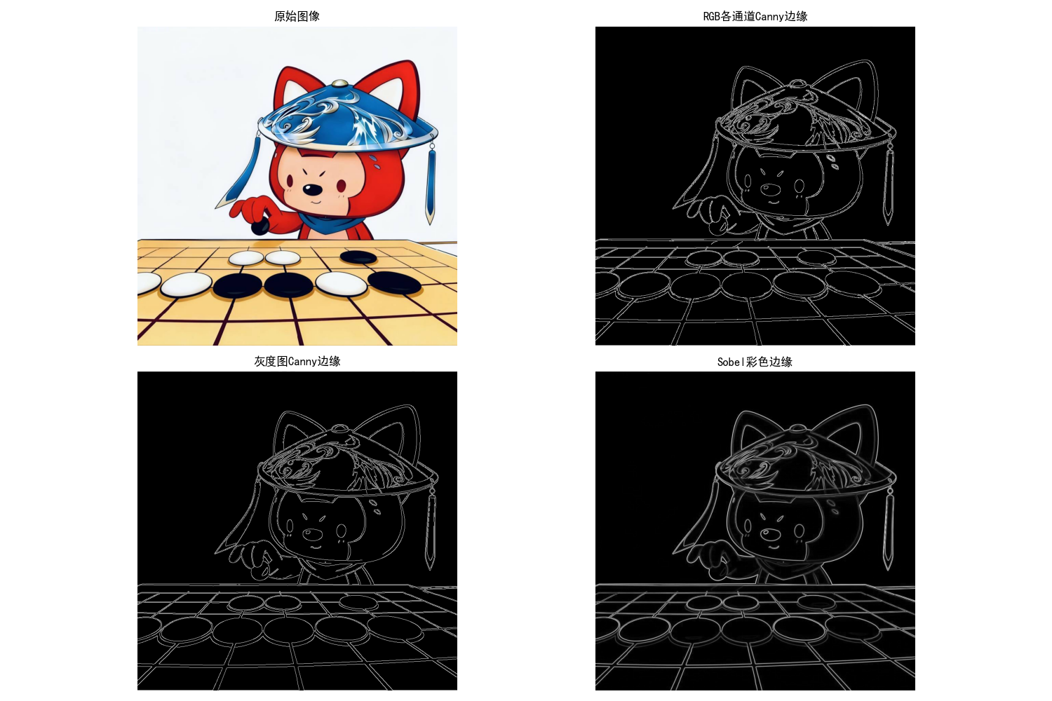
6.7.3 彩色边缘检测
检测彩色图像的边缘,可对各通道分别检测后合并,或直接处理RGB向量。
实战代码:彩色边缘检测
import cv2
import numpy as np
import matplotlib.pyplot as plt

plt.rcParams['font.sans-serif'] = ['SimHei']
plt.rcParams['axes.unicode_minus'] = False

# 彩色边缘检测
def color_edge_detection_demo():
    # 读取图像
    img = cv2.imread('test.jpg')
    img_rgb = cv2.cvtColor(img, cv2.COLOR_BGR2RGB)

    # 方法1:各通道分别Canny检测后合并
    r_edges = cv2.Canny(img_rgb[:, :, 0], 100, 200)
    g_edges = cv2.Canny(img_rgb[:, :, 1], 100, 200)
    b_edges = cv2.Canny(img_rgb[:, :, 2], 100, 200)
    rgb_edges = cv2.bitwise_or(cv2.bitwise_or(r_edges, g_edges), b_edges)

    # 方法2:转换为灰度图后Canny检测
    gray = cv2.cvtColor(img_rgb, cv2.COLOR_RGB2GRAY)
    gray_edges = cv2.Canny(gray, 100, 200)

    # 方法3:Sobel彩色边缘检测
    sobel_x = cv2.Sobel(img_rgb, cv2.CV_64F, 1, 0, ksize=3)
    sobel_y = cv2.Sobel(img_rgb, cv2.CV_64F, 0, 1, ksize=3)
    sobel_edges = np.sqrt(np.sum(sobel_x**2 + sobel_y**2, axis=-1))
    sobel_edges = (sobel_edges / np.max(sobel_edges) * 255).astype(np.uint8)

    # 可视化
    plt.figure(figsize=(15, 10))

    plt.subplot(2, 2, 1)
    plt.imshow(img_rgb)
    plt.title('原始图像')
    plt.axis('off')

    plt.subplot(2, 2, 2)
    plt.imshow(rgb_edges, cmap='gray')
    plt.title('RGB各通道Canny边缘')
    plt.axis('off')

    plt.subplot(2, 2, 3)
    plt.imshow(gray_edges, cmap='gray')
    plt.title('灰度图Canny边缘')
    plt.axis('off')

    plt.subplot(2, 2, 4)
    plt.imshow(sobel_edges, cmap='gray')
    plt.title('Sobel彩色边缘')
    plt.axis('off')

    plt.tight_layout()
    plt.show()

# 运行示例
if __name__ == '__main__':
    color_edge_detection_demo()
6.8 彩色图像噪声
彩色图像噪声会同时影响多个通道,常见噪声类型有高斯噪声、椒盐噪声、泊松噪声等。
实战代码:彩色图像噪声添加与去除
import cv2
import numpy as np
import matplotlib.pyplot as plt

plt.rcParams['font.sans-serif'] = ['SimHei']
plt.rcParams['axes.unicode_minus'] = False

# 彩色图像噪声添加与去除
def color_noise_demo():
    # 读取图像
    img = cv2.imread('test.jpg')
    img_rgb = cv2.cvtColor(img, cv2.COLOR_BGR2RGB)

    # 1. 添加高斯噪声
    gauss_noise = np.random.normal(0, 30, img_rgb.shape).astype(np.float32)
    img_gauss = img_rgb.astype(np.float32) + gauss_noise
    img_gauss = np.clip(img_gauss, 0, 255).astype(np.uint8)

    # 2. 添加椒盐噪声
    img_salt_pepper = img_rgb.copy()
    # 椒盐噪声比例
    s_vs_p = 0.5
    amount = 0.05
    # 生成噪声掩码
    out = np.zeros(img_rgb.shape, np.uint8)
    num_salt = np.ceil(amount * img_rgb.size * s_vs_p)
    coords = [np.random.randint(0, i - 1, int(num_salt)) for i in img_rgb.shape]
    img_salt_pepper[coords[0], coords[1], coords[2]] = 255
    num_pepper = np.ceil(amount * img_rgb.size * (1. - s_vs_p))
    coords = [np.random.randint(0, i - 1, int(num_pepper)) for i in img_rgb.shape]
    img_salt_pepper[coords[0], coords[1], coords[2]] = 0

    # 3. 去噪处理
    # 高斯噪声去噪:双边滤波
    denoise_gauss = cv2.bilateralFilter(img_gauss, 9, 75, 75)
    # 椒盐噪声去噪:中值滤波
    denoise_salt_pepper = cv2.medianBlur(img_salt_pepper, 3)

    # 可视化
    plt.figure(figsize=(15, 10))

    plt.subplot(3, 2, 1)
    plt.imshow(img_rgb)
    plt.title('原始图像')
    plt.axis('off')

    plt.subplot(3, 2, 2)
    plt.imshow(img_gauss)
    plt.title('添加高斯噪声')
    plt.axis('off')

    plt.subplot(3, 2, 3)
    plt.imshow(denoise_gauss)
    plt.title('高斯噪声去噪(双边滤波)')
    plt.axis('off')

    plt.subplot(3, 2, 4)
    plt.imshow(img_salt_pepper)
    plt.title('添加椒盐噪声')
    plt.axis('off')

    plt.subplot(3, 2, 5)
    plt.imshow(denoise_salt_pepper)
    plt.title('椒盐噪声去噪(中值滤波)')
    plt.axis('off')

    plt.tight_layout()
    plt.show()

# 运行示例
if __name__ == '__main__':
    color_noise_demo()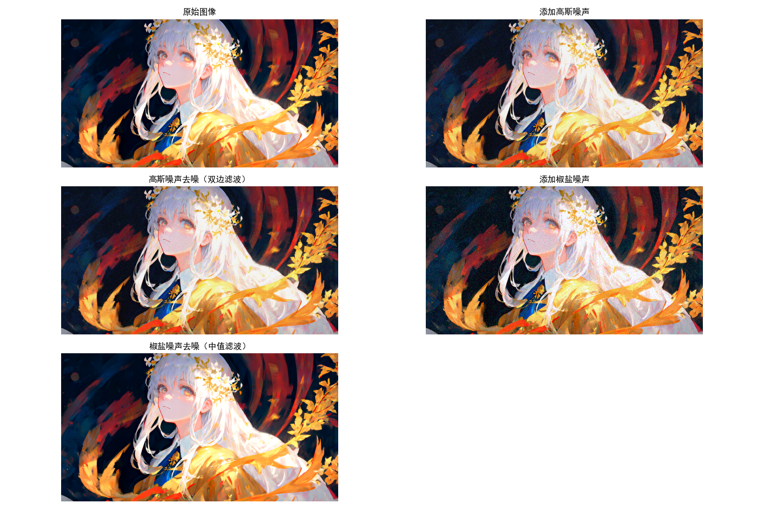
6.9 彩色图像压缩
彩色图像压缩是通过去除冗余信息(空间冗余、颜色冗余、视觉冗余)减少数据量,在保证视觉效果可接受的前提下,实现图像的高效存储与传输。常见压缩方式分为有损压缩(如JPEG)和无损压缩(如PNG),核心思路包括通道下采样、变换编码、熵编码等。
核心原理
-
颜色冗余去除:利用人眼对亮度敏感、对色度不敏感的特性,对色度通道(如Cb、Cr)进行下采样(如4:2:0格式),减少色度数据量。
-
变换编码:将图像从空间域转换到频率域(如DCT变换),对高频分量(细节)进行粗量化,保留低频分量(轮廓)。
-
熵编码:对量化后的数据进行无损压缩(如霍夫曼编码),进一步减少冗余。
实战代码:彩色图像压缩
import cv2
import numpy as np
import matplotlib.pyplot as plt
import os

# 设置matplotlib支持中文显示
plt.rcParams['font.sans-serif'] = ['SimHei']
plt.rcParams['axes.unicode_minus'] = False

def color_compression_demo():
    # 读取图像(替换为自己的图像路径,建议用相对路径)
    img_path = 'test.jpg'
    if not os.path.exists(img_path):
        print(f"提示:图像路径{img_path}不存在,可替换为本地图像路径")
        # 生成一张测试图备用
        img_rgb = np.zeros((400, 600, 3), dtype=np.uint8)
        img_rgb[:, :200] = [255, 0, 0]    # 红
        img_rgb[:, 200:400] = [0, 255, 0] # 绿
        img_rgb[:, 400:] = [0, 0, 255]    # 蓝
    else:
        img = cv2.imread(img_path)
        img_rgb = cv2.cvtColor(img, cv2.COLOR_BGR2RGB)

    # 1. JPEG有损压缩(不同质量对比)
    quality_levels = [90, 50, 10]  # JPEG质量(0-100,越高质量越好、体积越大)
    compressed_imgs = []
    compressed_sizes = []
    for q in quality_levels:
        # 编码为JPEG格式
        encode_param = [int(cv2.IMWRITE_JPEG_QUALITY), q]
        result, encimg = cv2.imencode('.jpg', cv2.cvtColor(img_rgb, cv2.COLOR_RGB2BGR), encode_param)
        # 解码回图像
        decimg = cv2.imdecode(encimg, cv2.IMREAD_COLOR)
        decimg_rgb = cv2.cvtColor(decimg, cv2.COLOR_BGR2RGB)
        compressed_imgs.append(decimg_rgb)
        # 记录压缩后大小
        compressed_sizes.append(len(encimg))

    # 2. 通道下采样压缩(4:2:0格式,模拟JPEG色度下采样)
    h, w = img_rgb.shape[:2]
    # 分离RGB通道
    r = img_rgb[:, :, 0]
    g = img_rgb[:, :, 1]
    b = img_rgb[:, :, 2]
    # 色度通道(G、B)下采样(宽高各缩小为1/2)
    g_down = cv2.resize(g, (w//2, h//2), interpolation=cv2.INTER_LINEAR)
    b_down = cv2.resize(b, (w//2, h//2), interpolation=cv2.INTER_LINEAR)
    # 上采样恢复尺寸(用于展示效果)
    g_up = cv2.resize(g_down, (w, h), interpolation=cv2.INTER_LINEAR)
    b_up = cv2.resize(b_down, (w, h), interpolation=cv2.INTER_LINEAR)
    # 组合成下采样后的图像
    subsampled_img = np.stack([r, g_up, b_up], axis=-1).astype(np.uint8)

    # 3. 计算压缩率(基于JPEG质量10的情况)
    original_size = len(cv2.imencode('.jpg', cv2.cvtColor(img_rgb, cv2.COLOR_RGB2BGR), [int(cv2.IMWRITE_JPEG_QUALITY), 100])[1])
    min_compressed_size = compressed_sizes[-1]
    compression_ratio = original_size / min_compressed_size  # 压缩比(越大压缩效果越好)

    # 可视化结果
    plt.figure(figsize=(16, 12))

    # 原始图像
    plt.subplot(2, 3, 1)
    plt.imshow(img_rgb)
    plt.title(f'原始图像\n(预估大小: {original_size/1024:.2f} KB)')
    plt.axis('off')

    # JPEG质量90
    plt.subplot(2, 3, 2)
    plt.imshow(compressed_imgs[0])
    plt.title(f'JPEG质量90\n(大小: {compressed_sizes[0]/1024:.2f} KB)')
    plt.axis('off')

    # JPEG质量50
    plt.subplot(2, 3, 3)
    plt.imshow(compressed_imgs[1])
    plt.title(f'JPEG质量50\n(大小: {compressed_sizes[1]/1024:.2f} KB)')
    plt.axis('off')

    # JPEG质量10
    plt.subplot(2, 3, 4)
    plt.imshow(compressed_imgs[2])
    plt.title(f'JPEG质量10\n(大小: {compressed_sizes[2]/1024:.2f} KB)')
    plt.axis('off')

    # 通道下采样
    plt.subplot(2, 3, 5)
    plt.imshow(subsampled_img)
    plt.title(f'4:2:0下采样图像\n(压缩比: {compression_ratio:.1f}:1)')
    plt.axis('off')

    plt.suptitle('彩色图像压缩效果对比', fontsize=14)
    plt.tight_layout()
    plt.show()

# 运行示例
if __name__ == '__main__':
    color_compression_demo()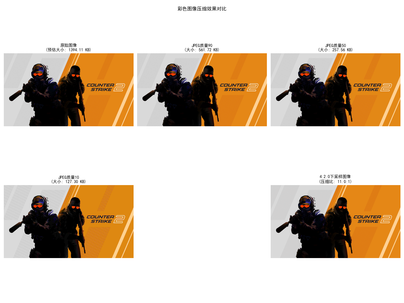
代码说明
-
JPEG压缩通过调整
IMWRITE_JPEG_QUALITY参数控制质量,质量10时体积最小但会出现块效应,质量90时视觉效果接近原图。 -
4:2:0下采样仅保留亮度通道(R)全分辨率,色度通道(G、B)分辨率减半,可减少50%的色度数据,且人眼几乎无法感知差异。
-
若本地无测试图,代码会自动生成RGB三通道测试图,确保可直接运行。
小结
本章围绕彩色图像处理的核心技术展开,从基础理论到实战应用,构建了完整的知识体系,核心要点可总结为以下几点:
1. 基础理论与颜色模型
色彩的本质是光的视觉感知,由亮度、色调、饱和度三要素决定。不同颜色模型适用于不同场景:RGB为加色模型,适配显示设备;CMY/CMYK为减色模型,适配印刷设备;HSI模型分离亮度与色彩信息,是彩色图像处理的首选模型,可有效避免亮度对色彩操作的干扰。
2. 伪彩色与真彩色处理
伪彩色处理通过灰度-颜色映射增强灰度图像细节,分为灰度分层法(离散着色)和灰度-颜色变换法(连续着色),适用于医学、遥感等领域。真彩色处理需兼顾通道一致性,可通过RGB通道独立操作或HSI空间分通道调整(如亮度、饱和度优化)实现效果增强。
3. 核心处理技术
彩色变换通过补色、色调校正、直方图均衡化等手段优化图像颜色与对比度,其中HSI空间亮度通道均衡化能获得更自然的增强效果。彩色平滑与锐化需避免颜色失真,平滑可采用高斯、中值滤波,锐化可通过Laplacian、USM算法实现,HSI空间锐化能精准保留色彩信息。
4. 高级应用场景
基于色彩的图像分割是目标提取的核心手段,HSI空间分割受光照影响小,稳定性优于RGB空间;RGB向量空间分割通过距离度量实现目标颜色提取,适用于简单场景。彩色图像噪声需针对性去噪,高斯噪声用双边滤波,椒盐噪声用中值滤波效果更佳。彩色压缩通过冗余去除实现高效存储,JPEG有损压缩是主流方案,通道下采样是减少数据量的关键手段。
5. 实战要点
彩色图像处理的核心是“分通道精准操作+跨空间协同优化”,需注意:OpenCV默认BGR格式,需转换为RGB后可视化;HSI与RGB的双向转换是实现复杂色彩操作的基础;所有实战代码均需考虑边界情况(如除以零、像素值溢出),通过clip函数和微小偏移量避免异常。
后续学习可结合深度学习(如彩色图像去噪、分割模型)进一步提升处理效果,彩色图像处理在计算机视觉、自动驾驶、医疗影像等领域的应用场景将持续拓展,掌握本章技术可为后续进阶学习奠定坚实基础。

DAMO开发者矩阵,由阿里巴巴达摩院和中国互联网协会联合发起,致力于探讨最前沿的技术趋势与应用成果,搭建高质量的交流与分享平台,推动技术创新与产业应用链接,围绕“人工智能与新型计算”构建开放共享的开发者生态。
更多推荐
 12
12 0
0- 0


 已为社区贡献8条内容

所有评论(0)