吴恩达机器学习课后习题1
3.成本函数和迭代函数。
·
# 吴恩达机器学习1-线性回归
- 首先导入库
import numpy as np
import pandas as pd
import matplotlib.pyplot as plt
- 读取数据集
##读取数据
datas = pd.read_csv('ex1data1.txt',names=['population','profit'])
print(datas.head())
print(datas.describe())
print(datas.info)
#原始数据页面绘图
print(datas.head())
datas.plot(kind='scatter', x='population', y='profit', figsize=(12, 8))
plt.show()
生成数据集图片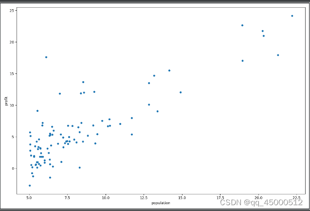
3. 成本函数和迭代函数
def costFunction(X,y,theta):
    inner =  np.power(X @ theta - y,2)
    return np.sum(inner) /(2*len(X))
def grandDescent(X,y,theta,alpha,iters):
    costs = []

    for i in range(iters):
        theta = theta - (X.T @ (X@theta - y)) * alpha/len(X)
        cost = costFunction(X,y,theta)
        costs.append(cost)

        if i % 100 == 0:
            print(cost)
    return theta,costs
- 绘制图片
#搞数据
datas.insert(0,'ones',1) #插入一行
X=datas.iloc[:,0:-1] ## 注意逗号相当于前两行切片
print(X.head())
X = X.values ##转换
print(X.shape) # 是什么行列 还有reshape
y = datas.iloc[:,-1]
y= y.values
y= y.reshape(97,1)
print(y.shape)
#迭代
theta=np.zeros((2,1))
theta.shape
cost_init=costFunction(X,y,theta)
print(cost_init)
alpha=0.02 # 学习率
iters=2000 #次数
theta,costs=grandDescent(X,y,theta,alpha,iters)
#绘图
#fig,ax = plt.subplots(2,3) # 2行3列 6个图
fig,ax = plt.subplots()
#散点图 scatter plot 是图
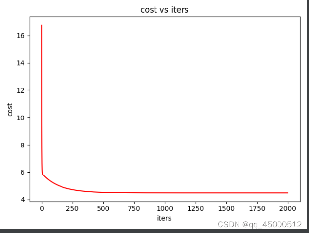
ax.plot(np.arange(iters),costs,'r') #最后是颜色 #costs是列表所以iters也得做成列表0,1,2到-1000
ax.set(xlabel='iters',
ylabel='cost',
title='cost vs iters')
#@ax.plot
plt.show()
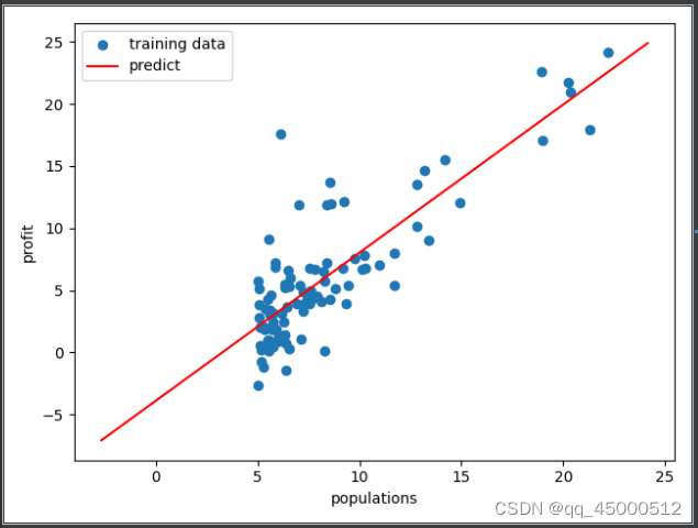
##综合图
x = np.linspace(y.min(),y.max(),100) ## 注意括号
y_ = theta[0,0]+theta[1,0]* x
fig,ax=plt.subplots()
ax.scatter(X[:,-1],y,label='training data')
ax.plot(x,y_,'r',label="predict")
ax.legend() ##让label生效
ax.set(xlabel='populations'
,ylabel='profit')
plt.show()
5. 知识点
数据差距过大梯度下降慢可以正规化
#特征归一化
def normalize_feature(data):
    return (data-data.mean()) / data.std()
少于10000数据可以用正规方法
def normalEquation(X,y):
    theta = np.linalg.inv(X.T@X)@X.T@y  ##正规方程法 类似于迭代
    return theta
设计不同学习率观看迭代效果
alphas=[0.0003,0.003,0.03,0.3,0.01] # 学习率
iters=2000 #次数
#不同学习率的迭代效果
fig,ax = plt.subplots()
for alpha in alphas:
    costs = grandDescent(X, y, theta, alpha, iters)
    ax.plot(np.arange(iters), costs, label=alpha)
    ax.legend()

ax.set(xlabel='iters',
       ylabel='cost',
       title='cost vs iters')
# @ax.plot
plt.show()
效果图 数据源另寻的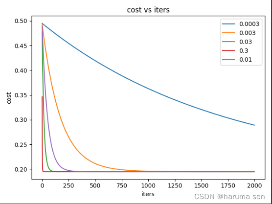
转换矩阵的三种方式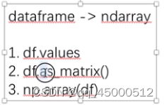

DAMO开发者矩阵,由阿里巴巴达摩院和中国互联网协会联合发起,致力于探讨最前沿的技术趋势与应用成果,搭建高质量的交流与分享平台,推动技术创新与产业应用链接,围绕“人工智能与新型计算”构建开放共享的开发者生态。
更多推荐


 1
1 0
0- 0


 已为社区贡献2条内容

所有评论(0)