When it comes to using machine learning in the stock market, there are multiple approaches a trader can do to utilize ML models. From determining future risk to predicting stock prices, machine learning can be used for virtually any kind of financial modeling.

它涉及到在股市中使用机器学习W¯¯母鸡，有多种方式交易者可以做到利用ML车型。 从确定未来风险到预测股票价格，机器学习几乎可以用于任何类型的财务建模。

In our previous articles, we delved into the usage of two Time Series models: SARIMAX and Facebook Prophet. We utilized both of these models to forecast the potential, future prices of Bitcoin. Check out the following article if you are interested:

在之前的文章中，我们深入研究了两个时间序列模型的用法： SARIMAX和Facebook Prophet 。 我们利用这两种模型来预测比特币的潜在未来价格。 如果您有兴趣，请查看以下文章：

In another article, we used classification models to classify stocks based on their performance in quarterly reports. You can read about the entire process of how we engineered different features from these reports and trained our classification models to determine investment decisions in the article below:

在另一篇文章中，我们使用分类模型根据股票在季度报告中的表现对股票进行分类。 您可以在以下文章中了解有关我们如何设计这些功能的不同功能以及训练我们的分类模型以确定投资决策的整个过程：

These are just a couple examples of how we can utilize machine learning models for financial markets.

这些只是我们如何在金融市场中利用机器学习模型的几个例子。

In these articles, we just used models to predict future prices, however, that is just half the battle. The next step is how do we evaluate these models if they were to actually be used while trading? The answer to that question is called — Backtesting.

在这些文章中，我们仅使用模型来预测未来价格，但这只是成功的一半。 下一步是如何在交易中实际使用这些模型时对其进行评估？ 该问题的答案称为-回测。

回测 (Backtesting)

What is backtesting? Backtesting is the process of applying a trading strategy, predictive model, or analytical method to historical data to evaluate its accuracy and performance.

什么是回测？ 回测是将交易策略，预测模型或分析方法应用于历史数据以评估其准确性和性能的过程。

It is very important to note that backtesting does not 100% accurately, represent live-trading in the past. However, you should only use it to inform your decision to live-trade your strategy or not. Even then, it may be more practical to forward-test your strategy before trading with real money.

非常重要的一点是要注意，回溯测试不能100％准确地表示过去的实时交易。 但是，您仅应使用它来告知您决定是否进行实时交易的决策。 即使这样，在使用真金白银进行交易之前，对您的策略进行前瞻性测试可能更为实用。

When we create a machine learning model, we need to backtest the model in order to determine how well it would have potentially performed in the past by feeding it historical data. There are two approaches when it comes to backtesting — Event-Driven and Vectorized Backtesting.

当我们创建机器学习模型时，我们需要对模型进行回测，以便通过提供历史数据来确定其在过去的潜在性能。 回溯测试有两种方法- 事件驱动和向量化回测。

向量化回测 (Vectorized Backtesting)

Today, we will be using vectorized backtesting in order to evaluate the performance of our machine learning model. This approach allows us to quickly observe how our ML model might have performed in the past. If you would like to learn more about vectorized backtesting, then we suggest reading the following article by a machine learning researcher which contributed to the outcome of this current project:

今天，我们将使用矢量化回测，以评估我们的机器学习模型的性能。 这种方法使我们能够快速观察过去ML模型的性能。 如果您想了解有关向量化回测的更多信息，那么我们建议阅读机器学习研究人员的以下文章，该文章为当前项目的成果做出了贡献：

编码我们的机器学习模型 (Coding Our Machine Learning Model)

In order to evaluate the performance of a machine learning model, we’ll first have to construct it in Python. The model we will be using is the AutoARIMA time series model from the pmdarima Python library. This model will quickly find the optimum parameters for us so we won’t need to worry about adjusting any modeling parameters.

为了评估机器学习模型的性能，我们首先必须在Python中构建它。 我们将使用的模型是pmdarima Python库中的AutoARIMA时间序列模型。 该模型将为我们快速找到最佳参数，因此我们无需担心调整任何建模参数。

However, if you do want to learn more about the parameters and what they mean, check out our previous article mentioned above that uses time series modeling to predict Bitcoin prices.

但是，如果您确实想了解有关参数及其含义的更多信息，请查看我们前面提到的使用时间序列建模来预测比特币价格的前一篇文章。

步骤1.导入必要的库 (Step 1. Importing Necessary Libraries)

import pandas as pd
import numpy as np
from pmdarima.arima import AutoARIMA
import plotly.express as px
import plotly.graph_objects as go
from tqdm.notebook import tqdm
from sklearn.metrics import mean_squared_error
from datetime import date, timedelta
import yfinance as yf

Each library here serves an important purpose for building and backtesting our ML model.

这里的每个库都为建立和回测我们的ML模型发挥了重要作用。

第2步。获取数据 (Step 2. Getting the Data)

# Getting the date five years ago to download the current timeframe
years = (date.today() - timedelta(weeks=260)).strftime("%Y-%m-%d")# Stocks to analyze
stocks = ['GE', 'GPRO', 'FIT', 'F']# Getting the data for multiple stocks
df = yf.download(stocks, start=years).dropna()# Storing the dataframes in a dictionary
stock_df = {}for col in set(df.columns.get_level_values(0)):
    
    # Assigning the data for each stock in the dictionary
    stock_df[col] = df[col]

The data we will be using is a small collection of stocks with about 260 weeks of historical data. To be even less biased towards the performance of our model, we used stocks that have decreased in value in the past few years.

我们将使用的数据是一小部分库存，其中包含大约260周的历史数据。 为了减少对模型性能的偏见，我们使用了过去几年中价值下降的股票。

步骤3.预处理数据 (Step 3. Preprocessing the Data)

# Finding the log returns
stock_df['LogReturns'] = stock_df['Adj Close'].apply(np.log).diff().dropna()# Using Moving averages
stock_df['MovAvg'] = stock_df['Adj Close'].rolling(10).mean().dropna()# Logarithmic scaling of the data and rounding the result
stock_df['Log'] = stock_df['MovAvg'].apply(np.log).apply(lambda x: round(x, 2))

First, we’ll get the log returns for ours stocks, which we used later on to determine overall returns. Next, a 10-day moving average was applied to the dataset in order to smooth out and reduce the noise in closing prices. Finally, we scaled the moving averages by using a logarithmic scale rounded to 2 decimal places.

首先，我们将获得股票的对数收益，之后将其用于确定总体收益。 接下来，将10天移动平均线应用于数据集，以平滑并减少收盘价中的噪音。 最后，我们使用对数标度四舍五入到小数点后两位来缩放移动平均值。

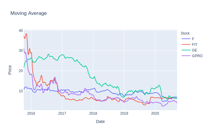
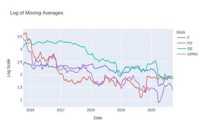
The reason we used moving averages and logarithmic scaling is because we hope that these values will be better suited for our model to predict prices much more accurately. There is no right answer in preprocessing or transforming the data to feed into our model so feel free to experiment with other scales, moving average windows, opening prices, etc.

我们使用移动平均和对数缩放的原因是，我们希望这些值将更适合我们的模型以更准确地预测价格。 在预处理或转换数据以馈入我们的模型中没有正确的答案，因此可以随意尝试其他比例，移动平均窗口，开盘价等。

步骤4.使用AutoARIMA进行训练和预测 (Step 4. Training and Predicting with AutoARIMA)

In order to run our model to get predictions with AutoARIMA, we will first layout all the requirements we want from our model and how to achieve them. Those things will be:

为了运行我们的模型以使用AutoARIMA进行预测，我们将首先布局模型中所需的所有需求以及如何实现它们。 这些事情将是：

• Number of days to train with — Let’s use about a half year’s worth of data from the past closing prices.

  需要培训的天数-让我们使用过去收盘价中大约半年的数据。

• Number of days to predict — Let’s predict the next 5 days into the future for our forecast amount and then use the last day as the price target for our trading strategy.

  可预测的天数-让我们预测未来5天的预测量，然后将最后一天用作我们交易策略的价格目标。

• When and how often will the model run — Let’s run the model every other day or whenever the current price reaches or passes the price target.

  模型的运行时间和频率-让我们每隔一天或当前价格达到或超过价格目标时运行模型。

• What date range we want to evaluate — We can set whatever range we like to backtest our ML model. Feel free to use whatever range you want but be aware that the bigger the range, the longer the training will take.

  我们要评估的日期范围-我们可以设置想要回测ML模型的任何范围。 随意使用您想要的任何范围，但要知道范围越大，训练所需的时间就越长。

All of these values can be tinkered with. Feel free to try out different values to potentially find an amount that works best with this trading strategy.

所有这些值都可以修改。 随时尝试不同的值，以潜在地找到最适合该交易策略的金额。

# Days in the past to train on
days_to_train = 180 


# Days in the future to predict
days_to_predict = 5


# Establishing a new DF for predictions
stock_df['Predictions'] = pd.DataFrame(index=stock_df['Log'].index,
                                       columns=stock_df['Log'].columns)


# Iterate through each stock
for stock in tqdm(stocks):
    
    # Current predicted value
    pred_val = 0
    
    # Training the model in a predetermined date range
    for day in tqdm(range(1000, 
                          stock_df['Log'].shape[0]-days_to_predict)):        


        # Data to use, containing a specific amount of days
        training = stock_df['Log'][stock].iloc[day-days_to_train:day+1].dropna()
        
        # Determining if the actual value crossed the predicted value
        cross = ((training[-1] >= pred_val >= training[-2]) or 
                 (training[-1] <= pred_val <= training[-2]))
        
        # Running the model when the latest training value crosses the predicted value or every other day 
        if cross or day % 2 == 0:


            # Finding the best parameters
            model    = AutoARIMA(start_p=0, start_q=0,
                                 start_P=0, start_Q=0,
                                 max_p=8, max_q=8,
                                 max_P=5, max_Q=5,
                                 error_action='ignore',
                                 information_criterion='bic',
                                 suppress_warnings=True)


            # Getting predictions for the optimum parameters by fitting to the training set            
            forecast = model.fit_predict(training,
                                         n_periods=days_to_predict)


            # Getting the last predicted value from the next N days
            stock_df['Predictions'][stock].iloc[day:day+days_to_predict] = np.exp(forecast[-1])




            # Updating the current predicted value
            pred_val = forecast[-1]

After we run the code above, we will be given a DF of predictions for every stock in our portfolio. We will use these predictions for our backtest but let’s visualize them first.

在运行完上面的代码之后，我们将获得投资组合中每只股票的DF预测。 我们将使用这些预测进行回测，但让我们首先对其进行可视化。

可视化模型的预测 (Visualizing the Model’s Predictions)

# Shift ahead by 1 to compare the actual values to the predictions
pred_df = stock_df['Predictions'].shift(1).astype(float).dropna()

Let’s create a new DataFrame for our predictions but with some alterations. We’ve shifted the predictions forward by one day so that our predictions will hopefully not suffer from look-ahead bias.

让我们为预测创建一个新的DataFrame，但要进行一些更改。 我们将预测提前了一天，这样我们的预测就不会遭受前瞻性偏差的困扰。

for stock in stocks:
    
    fig = go.Figure()
    
    # Plotting the actual values
    fig.add_trace(go.Scatter(x=pred_df.index,
                             y=stock_df['MovAvg'][stock].loc[pred_df.index],
                             name='Actual Moving Average',
                             mode='lines'))
    
    # Plotting the predicted values
    fig.add_trace(go.Scatter(x=pred_df.index,
                             y=pred_df[stock],
                             name='Predicted Moving Average',
                             mode='lines'))
    
    # Setting the labels
    fig.update_layout(title=f'Predicting the Moving Average for the Next {days_to_predict} days for {stock}',
                      xaxis_title='Date',
                      yaxis_title='Prices')
    
    fig.show()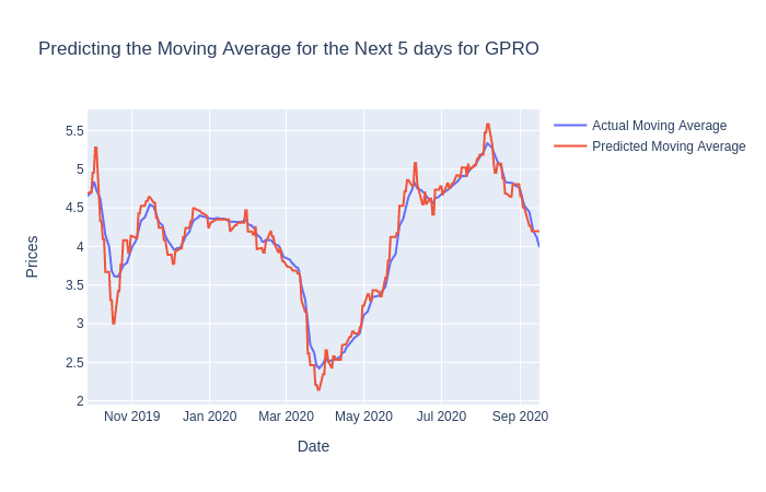

We can see that our model seems to do well enough but remember that the predictions are based on the last predicted day and serve as price targets in our trading strategy.

我们可以看到我们的模型似乎做得很好，但是请记住，这些预测是基于最后一个预测日，并且可以作为我们交易策略中的价格目标。

评估预测 (Evaluating the Predictions)

Now that we’ve seen the differences between the actual values and the predicted values, we can quickly evaluate it’s quality by using the Root Mean Square Error to see how far off our predictions are.

现在，我们已经看到了实际值和预测值之间的差异，我们可以通过使用均方根误差来查看预测值有多远，从而快速评估其质量。

for stock in stocks:
    
    # Finding the root mean squared error
    rmse = mean_squared_error(stock_df['MovAvg'][stock].loc[pred_df.index], pred_df[stock], squared=False)print(f"On average, the model is off by {rmse} for {stock}\n")

模型的交易策略 (The Trading Strategy for the Model)

Our strategy for our model is simple:

我们的模型策略很简单：

• Buy — When the predicted price target shows a significant increase from the current price.

  买—当预测价格目标显示比当前价格大幅上涨时。

• Sell — When the predicted price target shows a significant decrease from the current price.

  卖出—当预测价格目标显示比当前价格大幅下降时。

• Hold (or Do Nothing)— If the price target shows neither a significant increase or decrease from the current price.

  保留(或什么都不做)-如果价格目标与当前价格相比均未显示出明显的上升或下降。

For example: If we set our model to predict 10 days in advance, then the last day’s predicted amount is the price target. If the price target is $103 and the current closing price is $100, then we will buy that stock because its price is predicted to increase by 3% in the next 10 days.

例如：如果我们将模型设置为提前10天进行预测，则最后一天的预测金额就是价格目标。 如果目标价为103美元，当前收盘价为100美元，那么我们将购买该股票，因为预计其价格在未来10天内将上涨3％。

However, if the current price exceeds the predicted price target sooner than expected, then we can run the model again for a newer price target.

但是，如果当前价格比预期的价格更快地超出了预期的价格目标，那么我们可以为新的价格目标再次运行该模型。

Let’s create a function that will establish positions in our backtest based on the strategy above:

让我们创建一个函数，该函数将根据上述策略在回测中建立位置：

def get_positions(difference, thres=3, short=True):
    """
    Compares the percentage difference between actual 
    values and the respective predictions.
    
    Returns the decision or positions to long or short 
    based on the difference.
    
    Optional: shorting in addition to buying
    """
    
    if difference > thres/100:
        
        return 1
    
    
    elif short and difference < -thres/100:
        
        return -1
    
    
    else:
        
        return 0

基于模型预测的职位 (Positions Based on Model Predictions)

Now using our function to establish positions, we can begin the backtesting portion of our model and trading strategy. We will need to create another DataFrame containing the Log Returns to use and the percentage difference between our predicted and actual values.

现在使用我们的功能来建立头寸，我们可以开始模型和交易策略的回测部分。 我们将需要创建另一个DataFrame，其中包含要使用的Log Return以及预测值与实际值之间的百分比差异。

# Creating a DF dictionary for trading the model
trade_df = {}


# Getting the percentage difference between the predictions and the actual values
trade_df['PercentDiff'] = (stock_df['Predictions'].dropna() / 
                           stock_df['MovAvg'].loc[stock_df['Predictions'].dropna().index]) - 1


# Getting positions
trade_df['Positions'] = trade_df['PercentDiff'].applymap(lambda x: get_positions(x, 
                                                                                 thres=1, 
                                                                                 short=True) / len(stocks))


# Preventing lookahead bias by shifting the positions
trade_df['Positions'] = trade_df['Positions'].shift(2).dropna()


# Getting Log Returns
trade_df['LogReturns'] = stock_df['LogReturns'].loc[trade_df['Positions'].index]

If you noticed in the “Positions” DF, we have shifted the series of positions by 2 days. This is done to account for look-ahead bias as well as the situation in which we may find ourselves deciding to initiate a trade closer to the end of the trading day based on the prediction from the day before. If we decided to initiate a trade at the very beginning of the trading day, then we may be fine with just shifting positions by 1 day instead.

如果您在“位置” DF中注意到，我们已将一系列位置移动了2天。 这样做是为了考虑到前瞻性偏见以及可能基于前一天的预测而决定在交易日结束时开始进行交易的情况。 如果我们决定在交易日的开始时进行交易，那么将头寸转换1天就可以了。

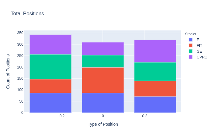
绘制位置 (Plotting the Positions)

Once we have established the positions in our backtest, we can then count the number of positions, the type of position, and which stock they belonged to. This is done to further analyze how often our strategy determines each position.

一旦在回测中建立了头寸，我们就可以计算头寸的数量，头寸的类型以及它们所属的股票。 这样做是为了进一步分析我们的策略确定每个职位的频率。

向量化回测模型 (Vectorized Backtesting the Model)

With our trading DataFrame ready to go, we can use vectorized backtesting and quickly visualize the returns for each individual stock and the returns from the overall portfolio.

准备好交易数据框架后，我们可以使用向量化回测，并快速可视化每只股票的收益和整个投资组合的收益。

每只股票的收益 (Returns for Each Stock)

# Calculating Returns by multiplying the 
# positions by the log returns
returns = trade_df['Positions'] * trade_df['LogReturns']# Calculating the performance as we take the cumulative 
# sum of the returns and transform the values back to normal
performance = returns.cumsum().apply(np.exp)# Plotting the performance per stock
px.line(performance,
        x=performance.index,
        y=performance.columns,
        title='Returns Per Stock Using ARIMA Forecast',
        labels={'variable':'Stocks',
                'value':'Returns'})

This code yields the following output for our vectorized backtest:

此代码为我们的向量化回测产生以下输出：

From this visualization, we can see that our ARIMA model strategy performs better with some stocks compared to others. With most of the stocks, you can see a significant jump right around March due to COVID’s effect on the market.

从该可视化中，我们可以看到，与其他股票相比，我们的ARIMA模型策略在某些股票上的表现更好。 对于大多数股票，由于COVID对市场的影响，您可以看到三月份左右的大幅上涨。

投资组合收益 (Returns on the Portfolio)

In order to really evaluate our portfolio returns, we will need to compare our results with SPY. If we are capable of beating SPY returns, then our model shows promise and may be considered for forward-testing or live trading.

为了真正评估我们的投资组合收益，我们需要将我们的结果与SPY进行比较。 如果我们有能力击败SPY回报，那么我们的模型将显示出希望，并可以考虑用于远期测试或实时交易。

# Returns for the portfolio
returns = (trade_df['Positions'] * trade_df['LogReturns']).sum(axis=1)


# Returns for SPY
spy = yf.download('SPY', start=returns.index[0]).loc[returns.index]


spy = spy['Adj Close'].apply(np.log).diff().dropna().cumsum().apply(np.exp)


# Calculating the performance as we take the cumulative sum of the returns and transform the values back to normal
performance = returns.cumsum().apply(np.exp)


# Plotting the comparison between SPY returns and ARIMA returns
fig = go.Figure()


fig.add_trace(go.Scatter(x=spy.index,
                         y=spy,
                         name='SPY Returns',
                         mode='lines'))


fig.add_trace(go.Scatter(x=performance.index,
                         y=performance.values,
                         name='ARIMA Returns on Portfolio',
                         mode='lines'))


fig.update_layout(title='SPY vs ARIMA Overall Portfolio Returns',
                  xaxis_title='Date',
                  yaxis_title='Returns')


fig.show()

And here’s the result:

结果如下：

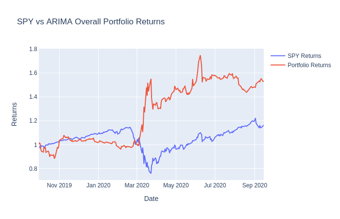
As you can see, our model initialy under-performs when compared to the SPY returns. However, it begins to beat SPY at the start of the stock market crash due to COVID. Feel free to change several values here and there within the model and within the strategy if you wish to achieve a different outcome.

如您所见，与SPY回报相比，我们的模型初始表现不佳。 但是，由于COVID，在股市崩盘之初它就开始击败SPY。 如果您希望获得不同的结果，请随时在模型内和策略内随时更改几个值。

总结思想 (Closing Thoughts)

When we used this AutoARIMA model in combination with our simple stock trading strategy, we were able to achieve a better return performance than if we had just invested in SPY. However, we were able to perform pretty well at the end possibly due to the sudden stock market crash.

当我们将此AutoARIMA模型与简单的股票交易策略结合使用时，与仅仅投资于SPY相比，我们可以获得更好的回报。 但是，由于股市突然暴跌，我们最终还是表现不错。

If we backtested on a different time frame or with different stocks, then it’s very probable we would not have achieved similar results. At this point, it’s a smart move to begin forward-testing this strategy in order to gain a better understanding of our model’s true performance.

如果我们在不同的时间范围内或使用不同的股票进行回测，那么很有可能我们不会取得相似的结果。 在这一点上，明智的做法是开始对该策略进行正向测试，以便更好地了解我们模型的真实性能。

资源资源 (Resources)