吴恩达机器学习[7]-Logistic回归算法-介绍与python实现
Logistic回归算法-介绍与python实现
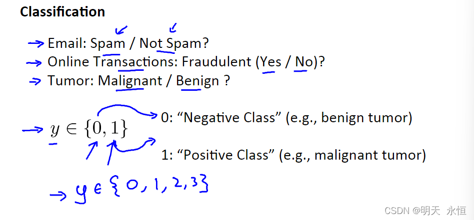
分类
分类预测算法
y存在两个取值,即0、1。【y取值为0,1,2或更多时,为多分类问题。】
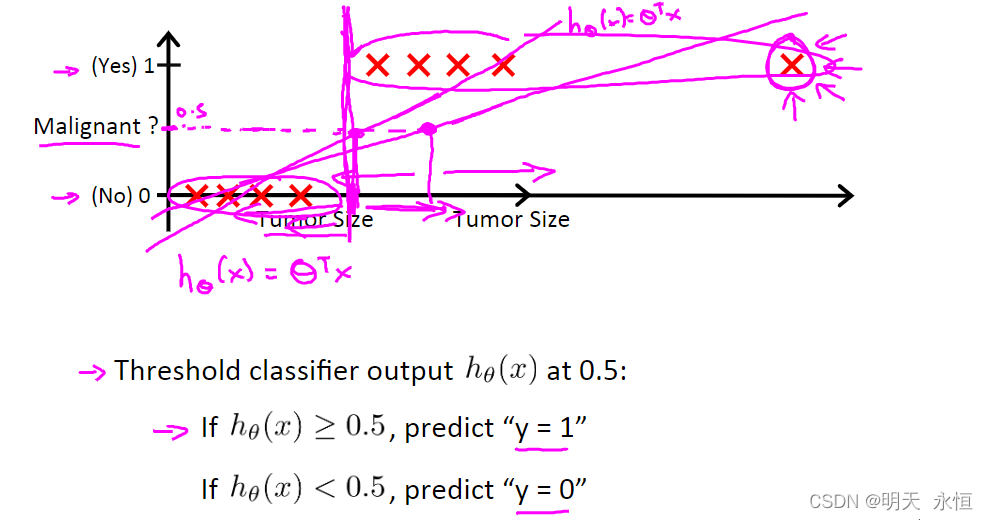
此时,简单的线性回归加上阈值划分,无法很合拟合点分布。
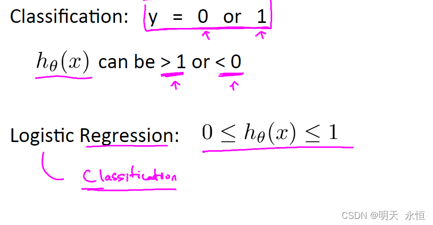
因此,引入logistic回归算法。‘回归’二字是历史原因导致,本算法属于分类算法。
假设陈述
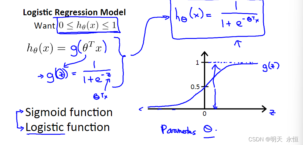
y的取值为[0,1]。为此引入sigmoid函数g(z),又称logistic函数。用该函数代入
h
θ
(
x
)
h_{\theta}(x)
hθ(x).用该函数拟合系列点。
模型解释
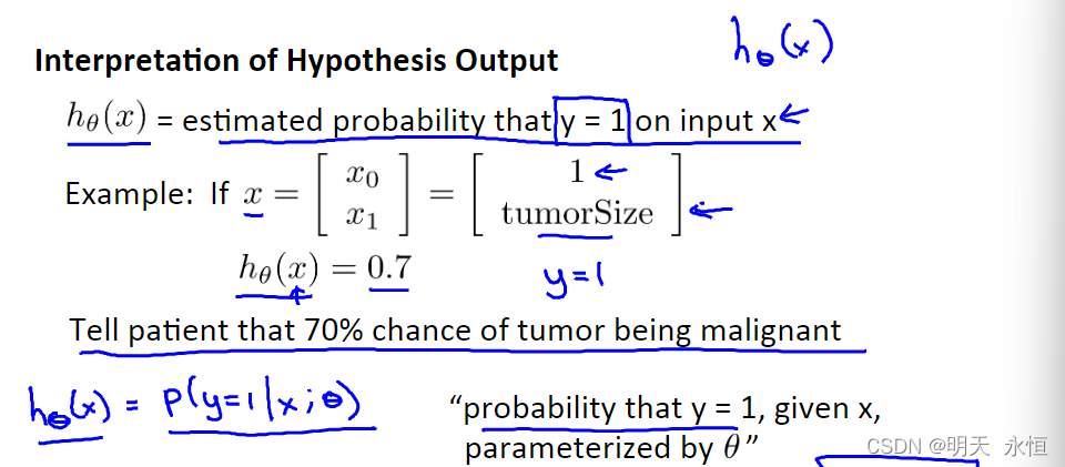
该模型可以理解为:在给定条件x的情况下,y=1的概率。其中概率参数为
θ
\theta
θ。代入肿瘤问题,即病人的特征为x的情况下,x代表肿瘤大小。
性质

决策边界
目标
- 了解决策边界(desicion boundary)定义
- 通过决策边界更好地理解logistic回归函数的假设函数在计算什么
根据sigmoid函数可看出,当
θ
T
x
\theta^{T}x
θTx大于等于0时,预测y等于0。总之,我们预测y等于0或1,取决于
θ
T
x
\theta^{T}x
θTx大于0还是小于0。
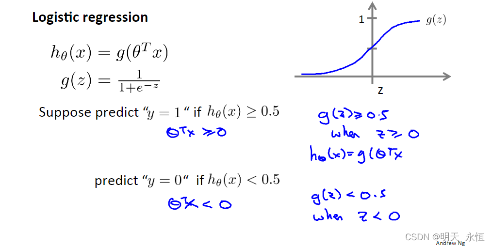
那么可以得出,假设函数如何做出预测。
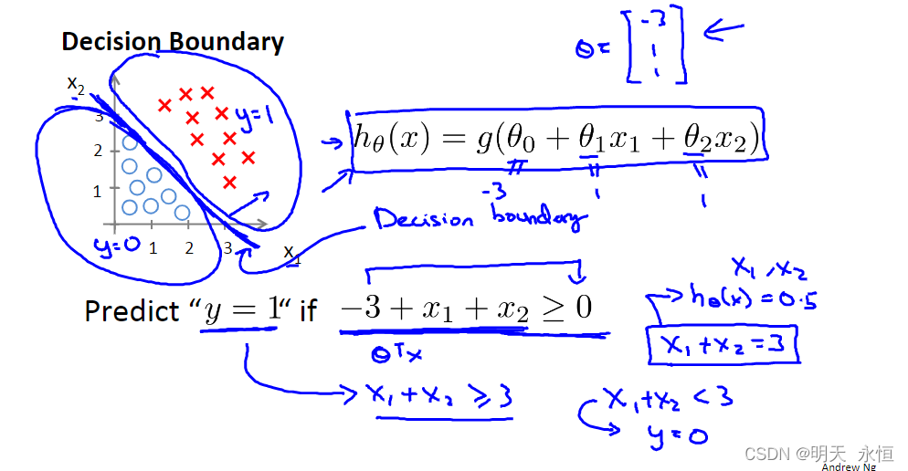
假设有如下函数。那么
−
3
+
x
1
+
x
2
+
x
3
≥
0
-3+x_{1}+x_{2}+x_{3}≥0
−3+x1+x2+x3≥0时,预测y为1,对应红x对应区域。相应地,可以得到预测y为0对应区域。两区域中间的线被称为决策边界(desicion boundary),直线上的点对应y为0.5。
需要注意的是,决策边界为假设函数的一个属性,它包括参数
θ
0
、
θ
1
、
θ
2
\theta_{0}、\theta_{1}、\theta_{2}
θ0、θ1、θ2。决策边界,包括预测y=0、y=1对应与区域,决定于其参数,它不是数据集的属性。
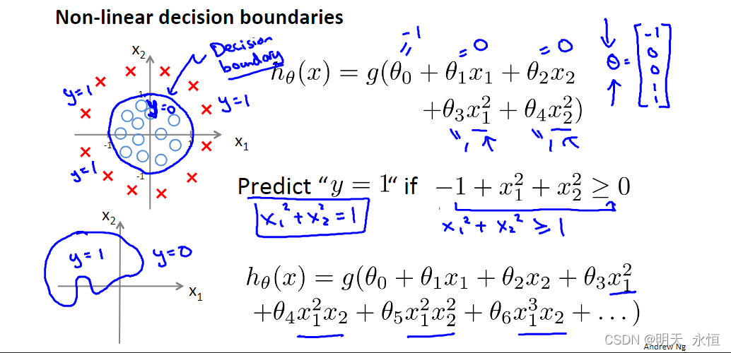
进化到更高阶的假设函数,原理也是同前者。蓝线圆圈代表决策边界。
代价函数
目标
- 如何拟合logistics回归函数的模型参数 θ \theta θ,即定义用来拟合参数的代价函数(优化目标)
给定训练集,设置样本的第一个变量值
x
0
x_{0}
x0为0,求
θ
\theta
θ
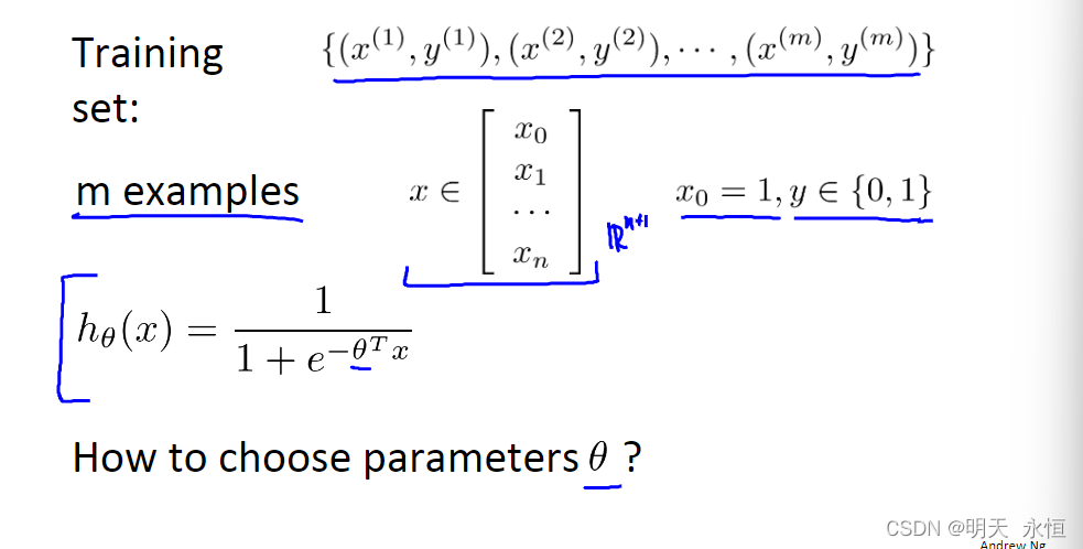
定义代价函数
J
(
θ
)
J(\theta)
J(θ),将求和函数内多项式定义为函数
c
o
s
t
(
h
θ
(
x
i
,
y
i
)
cost(h_\theta (x^{i} ,y^{i})
cost(hθ(xi,yi)。求代价函数最小值,即求
c
o
s
t
(
h
θ
(
x
i
,
y
i
)
cost(h_\theta (x^{i} ,y^{i})
cost(hθ(xi,yi)函数最小值。
但该函数为非凸函数(non-convex),存在很多局部最小值。使用梯度下降法不能保证获得全局局部最小值。
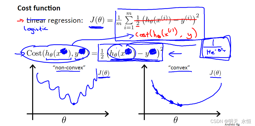
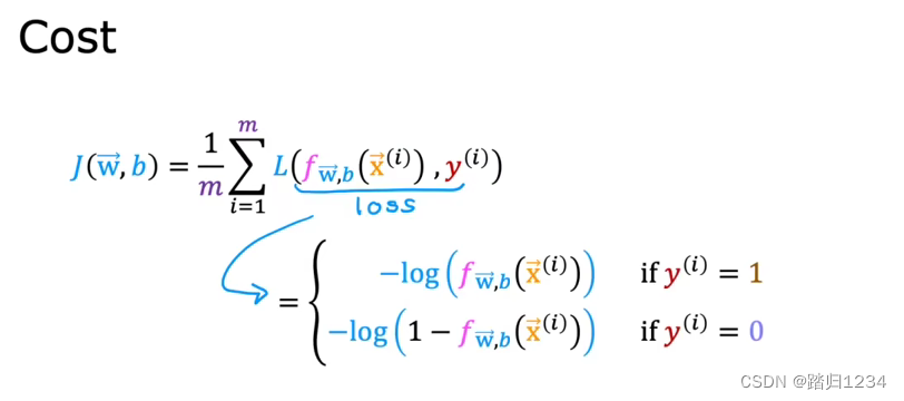
因此需要找到一个能使用梯度下降法的代价函数。因此找到如下代价函数。通过极大似然法求得。他是统计学中为不同函数快速寻找参数的方法,如何求???
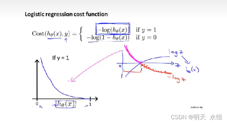
函数性质
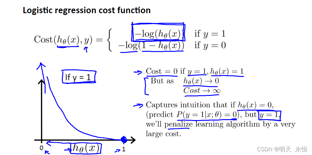
- y为1,
h
θ
(
x
)
h_\theta (x)
hθ(x)为1时,cost为0;但
h
θ
(
x
)
h_\theta (x)
hθ(x)趋向于0时,cost趋向于无限大。因此
h
θ
(
x
)
h_\theta (x)
hθ(x)为1时,y需要为1,不然得付出极大代价。
- y为0,
h
θ
(
x
)
h_\theta (x)
hθ(x)为0时,cost为0;但
h
θ
(
x
)
h_\theta (x)
hθ(x)趋向于1时,cost趋向于无限大。因此
h
θ
(
x
)
h_\theta (x)
hθ(x)为0时,y需要为0,不然得付出极大代价。
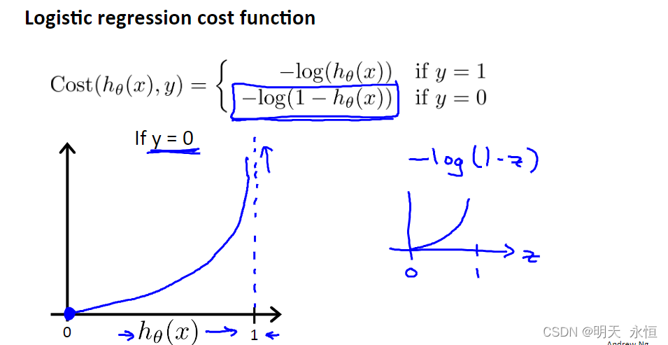
总之,因为逻辑回归代价函数使用均方误差时,代价函数为非凸函数。因此,构造一个新的代价函数。此时,代价函数为凸函数,且满足逻辑回归模型求解要求。
简化代价函数与梯度下降
目标
- 如何用更简单的方法写代价函数
- 如何利用梯度下降方法拟合logistic回归的参数
- 实现一个完整的logistic回归算法
定义新代价函数替代原本函数
c
o
s
t
(
h
θ
(
x
,
y
)
=
−
y
l
o
g
(
h
θ
(
x
)
−
(
1
−
y
)
l
o
g
(
1
−
h
θ
(
x
)
)
cost(h_\theta (x ,y)=-ylog(h_\theta (x)-(1-y)log(1-h_\theta (x))
cost(hθ(x,y)=−ylog(hθ(x)−(1−y)log(1−hθ(x))
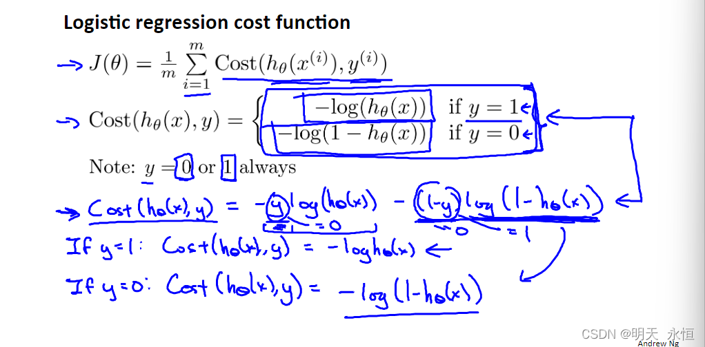
将上述函数代入
J
(
θ
)
J(\theta)
J(θ)函数,所以最终目标即求的最小值
l
i
m
θ
J
(
θ
)
\underset{\theta}{lim} J(\theta)
θlimJ(θ)。
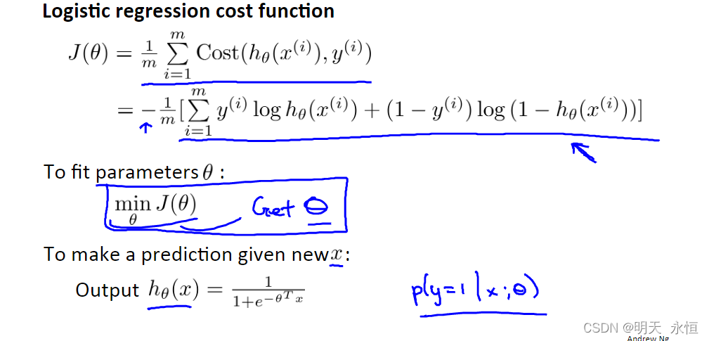
此函数为凸函数,因此可以使用梯度下降法。(
g
′
(
x
)
=
g
(
x
)
∗
(
1
−
g
(
x
)
)
g'(x)=g(x)*(1-g(x))
g′(x)=g(x)∗(1−g(x)))
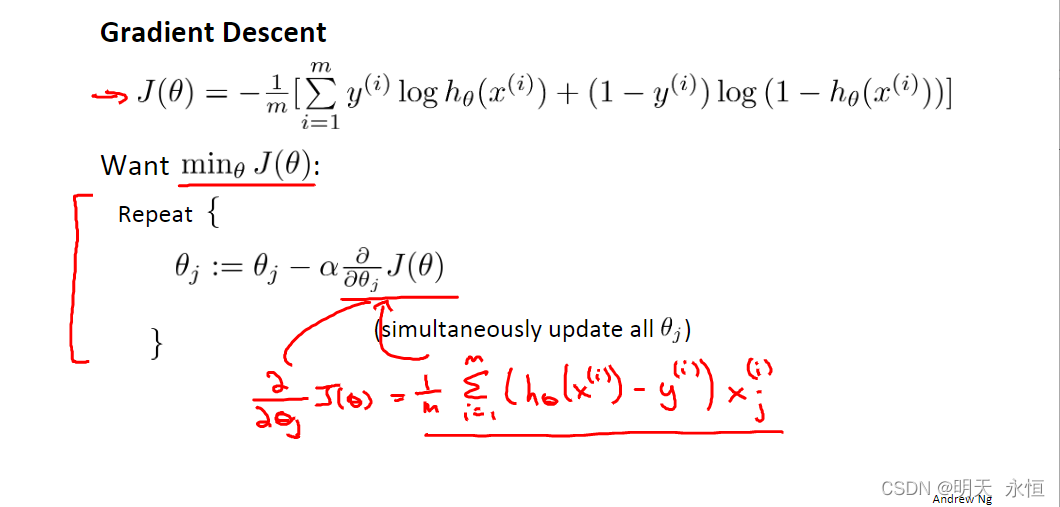
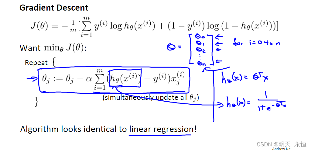
直接代入梯度下降的求导公式,得到公式如下。与多元线性回归参数计算公式类似,但性质完全不一样。因为假设函数
h
θ
(
x
i
)
h_\theta (x^{i})
hθ(xi)不同。
高级优化
目标
- 优化logistic回归算法计算速度
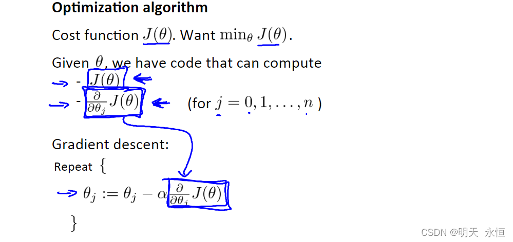
logistic求参,即代价函数 J ( θ ) J(\theta) J(θ)求最小值,可用梯度下降
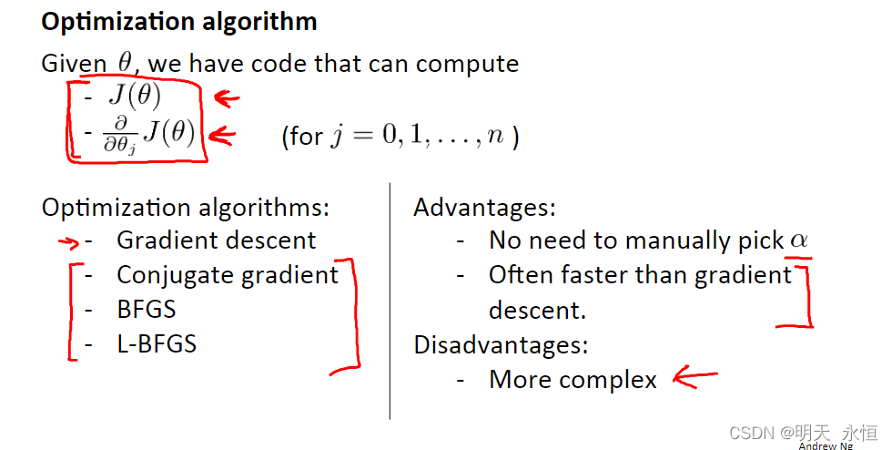
最小化代价函数方法包括梯度下降、BFGS等
多元分类:一对多
目标
- 如何将逻辑回归分类用在多元分类问题上。
多分类问题:y可以取1,2,3,4等离散值
下面以包括三个类别多元分类问题为例介绍,
将其划分为三个二分类问题,分别拟合三个分类器。对于每个分类器将小类当做正类别,因此x(1)实际是计算给定x和
θ
\theta
θ时y=1概率(三角形所在分类器);x(2)……y=2。
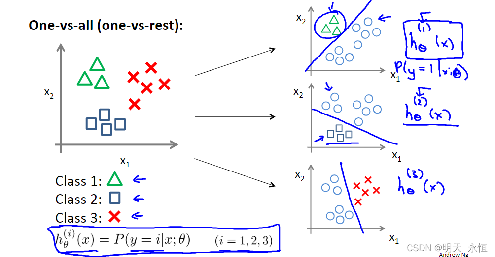
总之,我们将多元分问题划分为多个二元分类问题,分别计算各分类器的
h
θ
(
i
)
(
x
)
h_{\theta}^{(i)}(x)
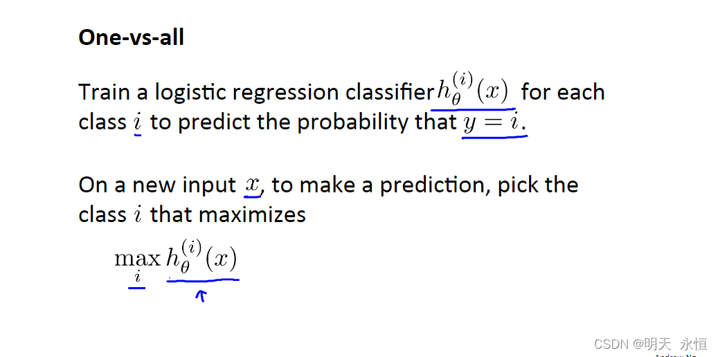
hθ(i)(x),值最大(也就是概率最大)即为最终被分的类别。
总结与代码实现
Logistic回归与线性回归差异
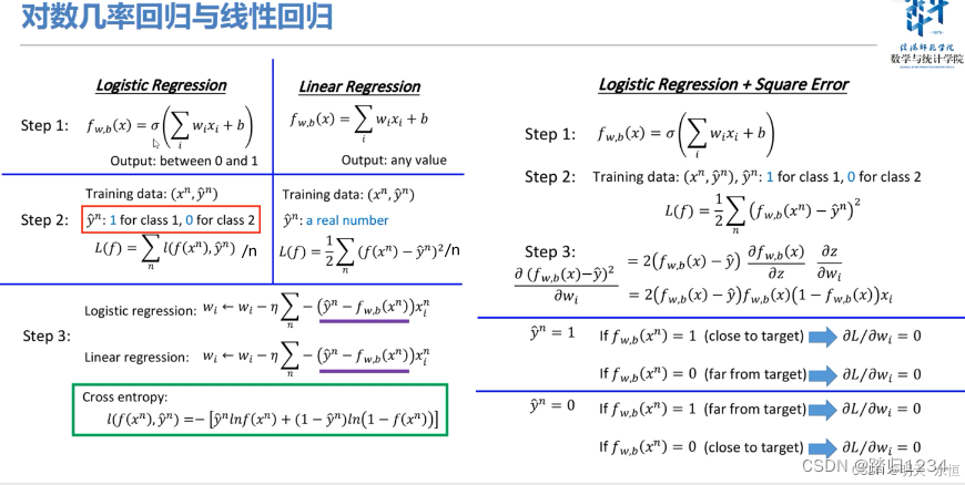
- Logistic回归函数 分类函数,加一个sigmoid函数(神经网络中叫激活函数);目标值为离散值,即类别;损失函数采用交叉熵损失函数
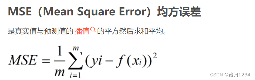
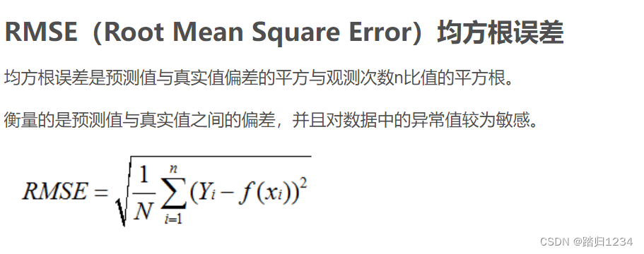
- Linear回归函数 目标值为任意实数;损失函数采用均方误差
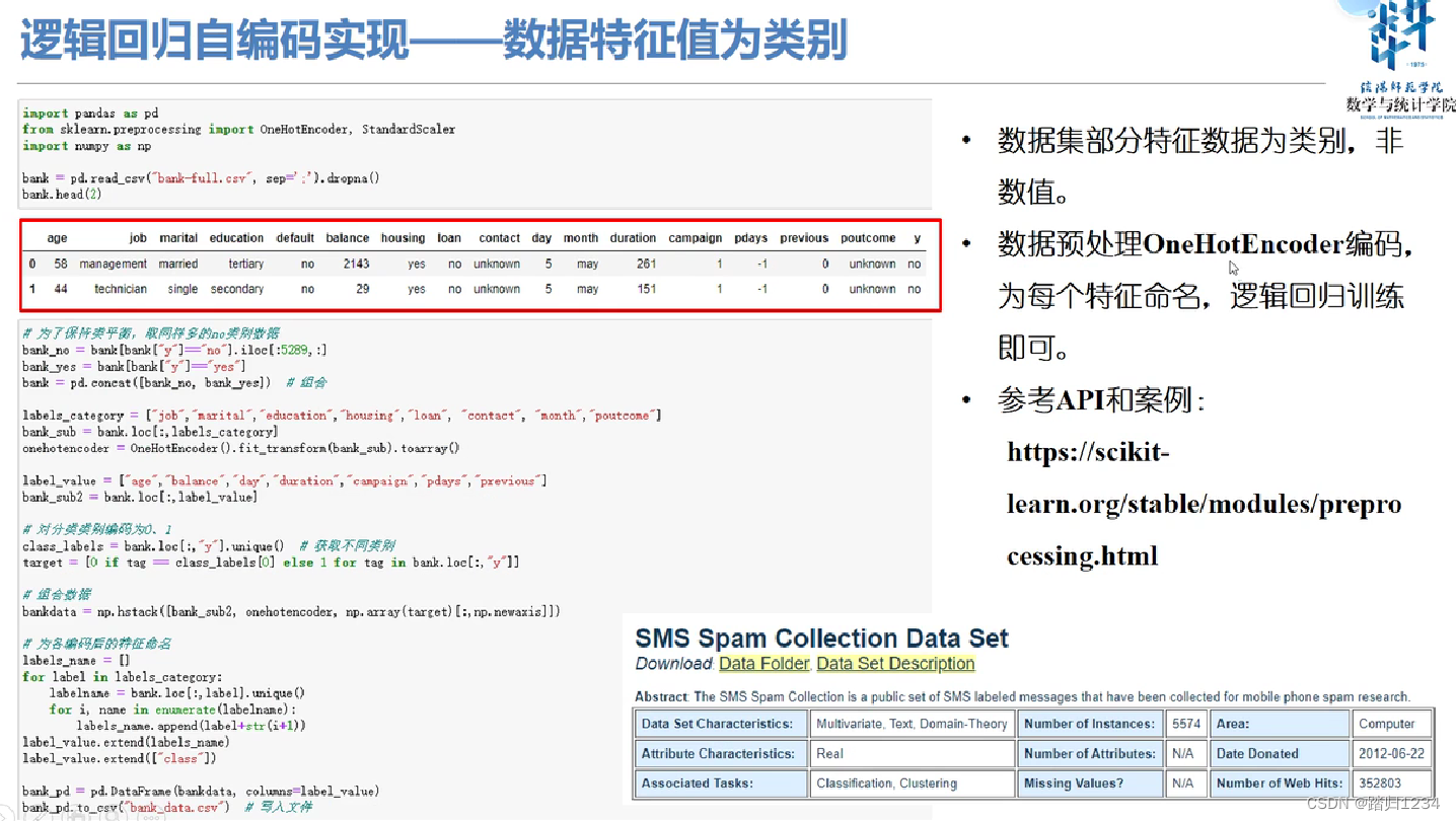
数据特征值为类别的处理
Logictic回归代码实现(Python)

"logistic regression"
import pandas as pd
import numpy as np
import matplotlib.pyplot as plt
import seaborn as sns
from sklearn.model_selection import train_test_split
from sklearn.preprocessing import StandardScaler#标准化
from sklearn.metrics import confusion_matrix,roc_curve,auc,classification_report #分类度量方法

class logisticRegressionGradientDescent:
    """
    逻辑回归,采用批量梯度下降,交叉熵损失函数
    """
    def __init__(self,dataset,attribute_list,aplha):
        """
        类初始化
        :param dataset:数据集
        :param attribute_list:特征列表
        :param aplha:学习率
        """
        self.alpha=aplha
        self.attr_list =attribute_list[:-1]#特征值
        self.target_lable=attribute_list[-1]#目标列名(取最后一列)
        #数据标准化
        self.X= StandardScaler().fit_transform(dataset.iloc[:,:-1])
        #对目标值进行编码
        self.y,self.class_lables = self.target_encode(dataset.iloc[:,-1])
        #划分数据集,分层抽样(stratify 按照列标y) random_state随机种子,防止每次运行结果重现
        self.x_train,self.x_test,self.y_train,self.y_test=\
            train_test_split(self.X,self.y,train_size=0.8,random_state=1,stratify=self.y)
        self.n,self.k=self.x_train.shape #训练数据样本量,特征变量个数
        self.cross_entropy_cost = []#每次训练交叉熵的平均值
        self.bdg_weight= dict()#每次训练权重更新

    @staticmethod
    def sigmoid(y_preval):
        '''
        激活函数
        :param y_preval: 样本值乘以权重系数后的值,数组
        :return:
        '''
        return 1/(1+np.exp(-y_preval))
    @staticmethod
    def target_encode(target):
        """
        静态方法,不用self,标记 @staticmethod
        二分类类别编码为0,1
        :param self:
        :param target: 类别列表
        :return:
        """
        class_lables=target.unique()# 获取不同类别值
        if len(class_lables)>2:
            print("此逻辑回归只是限于二分类,请选择多分类算法")
            exit(0)
        if(class_lables.max()==1 and class_lables.min()==0):
            return target.tolist(),class_lables
        else:
            #编码,采用列表推导式
            target_y = [0 if y == class_lables[0] else 1 for y in target]
            return target_y,class_lables

    def logistic_regression_model_train(self,max_lop,threshold):
        '''
        逻辑回归训练函数,采用批量梯度下降法,交叉熵损失函数
        :param max_lop: 最大训练次数
        :param threshold:退出训练阈值
        :return:
        '''
        np.random.seed(101)#设置随机种子,避免每次都一样
        weight =np.random.random(self.k)/100 #随机化权重 权重数同特征变量数  random模块的random函数
        weight_old =weight

        for j in range(self.k):
            self.bdg_weight[str(j)]=[]
        for loop in range(max_lop):
            self.alpha*=0.95#衰减指数慢慢减少
            y_hat = self.sigmoid(self.x_train.dot(weight.T))#激活函数·,预测属于某一类别的概率(0,1) 求x乘以权重 矩阵计算
            dw= ((y_hat-self.y_train)*self.x_train.T).mean(axis=1)#权值更新 对所有的列求均值 结果等同于(self.x_train.T*(y_hat-self.y_train)).mean(axis=1)
            weight=weight-self.alpha*dw #权值更新
            for j in range(self.k):
                self.bdg_weight[str(j)].append(weight[j])
            #交叉熵损失均值 1e-10是因为防止log后取值太小对结果产生影响
            ce_loss =-(np.array(self.y_train)*np.log(y_hat+1e-10)+
                       (1-np.array(self.y_train))*np.log(1-y_hat+1e-10)).mean()
            self.cross_entropy_cost.append(ce_loss)
            #退出条件,避免过拟合,提前停止训练
            if(len(self.cross_entropy_cost)>2):
                if np.abs(self.cross_entropy_cost[-1]-self.cross_entropy_cost[-2])>threshold:
                    break
                elif np.abs(weight-weight_old).all()<threshold:
                    break
                else:
                    weight_old=weight
        # #画图
        # plt.plot(self.cross_entropy_cost)
        # plt.show()
        return weight

    def plt_cost(self):
        """
        绘制交叉熵损失下降曲线
        :return:
        """
        plt.plot(self.cross_entropy_cost)
        plt.xlabel("Training times")
        plt.ylabel("Cross entropy cost")
        plt.title("Decline curve of loss function in Logistic regression")
        # plt.show()

    def plt_weight(self):
        """
        绘制权重更新曲线
        :return:
        """
        for k in range(self.k):
            plt.plot(self.bdg_weight[str(k)],label=self.attr_list[k])
        plt.legend()
        plt.xlabel("Training times")
        plt.ylabel("Weight")
        plt.title("Logistic regression weight coefficient update curve")

    def predict(self,weight):
        """
        测试样本预测类别,并根据概率进行类别编码
        :param weight:训练最终权重
        :return:
        """
        y_pred =[]#预测类别
        y_score =self.sigmoid(self.x_test.dot(weight.T))
        threshold =0.5 # 类别不平衡问题需要考虑阈值,待解决
        for y in y_score:
            if y<threshold:
                y_pred.append(0)
            elif y>= threshold:
                y_pred.append(1)
        cm= confusion_matrix(self.y_test,y_pred)
        acc= np.sum(np.diag(cm))/len(y_pred) #预测精度
        return y_pred,cm,acc,y_score

    def plt_confusion_matrix(self,cm,acc):
        """
        绘制混淆矩阵
        :param cm: 混淆矩阵
        :param acc: 预测精度
        :return:
        """
        cm =pd.DataFrame(cm,columns=self.class_lables,index=self.class_lables)
        sns.heatmap(cm,annot=True,cbar=False,fmt='d')#绘制热图
        plt.xlabel("Predict")
        plt.ylabel("True")
        plt.title("Confusion matrix and accuracy =%.2f%%" %(acc*100))#%%表示直接输出一个%

    def plt_roc_auc(self,y_score):
        """
        绘制ROC曲线,并计算AUC
        :param y_score: 预测样本预测评分
        :return:
        """
        false_positive_rate,true_positive_rate,_ =roc_curve(self.y_test,y_score)
        roc_auc=auc(false_positive_rate,true_positive_rate)
        plt.plot(false_positive_rate,true_positive_rate,"b",label="AUC=%.2f" % roc_auc)
        plt.legend(loc="lower right")
        plt.plot([0,1],[0,1],"r--")
        plt.xlabel("False_positive_rate")
        plt.ylabel("True_positive_rate")
        plt.title("Logistic Regression of Binary Classification ROC Curve and AUC")

if __name__=='__main__':
    url="../datasets/Mtrain_set.csv"#数据集路径
    data=pd.read_csv(url).dropna().iloc[:,1:]
    attribute_list =data.columns#列名列表  list列表,没有loc属性
    alpha =0.8
    #print(attribute_list)
    lrgd=logisticRegressionGradientDescent(data,attribute_list,alpha)
    weight=lrgd.logistic_regression_model_train(1000,1e-8)
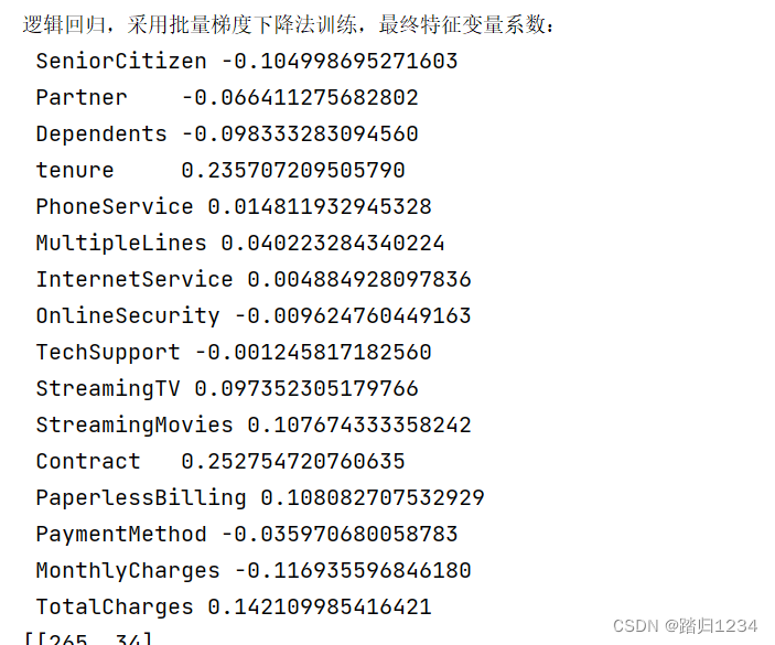
    print("逻辑回归,采用批量梯度下降法训练,最终特征变量系数:")
    for i in range(lrgd.k):
        print(" %-10s %.15f" % (lrgd.attr_list[i],weight[i]))
    y_pred,cm,acc,y_score =lrgd.predict(weight)
    #绘图
    plt.figure(figsize=(12,10))
    plt.subplot(221)#表示将整个图像窗口分为2行2列, 当前位置为1.
    lrgd.plt_cost()
    plt.subplot(222)
    lrgd.plt_weight()
    plt.subplot(223)
    lrgd.plt_confusion_matrix(cm,acc)
    plt.subplot(224)
    lrgd.plt_roc_auc(y_score)
    plt.show()

    #还可以再打印出一个分类报告
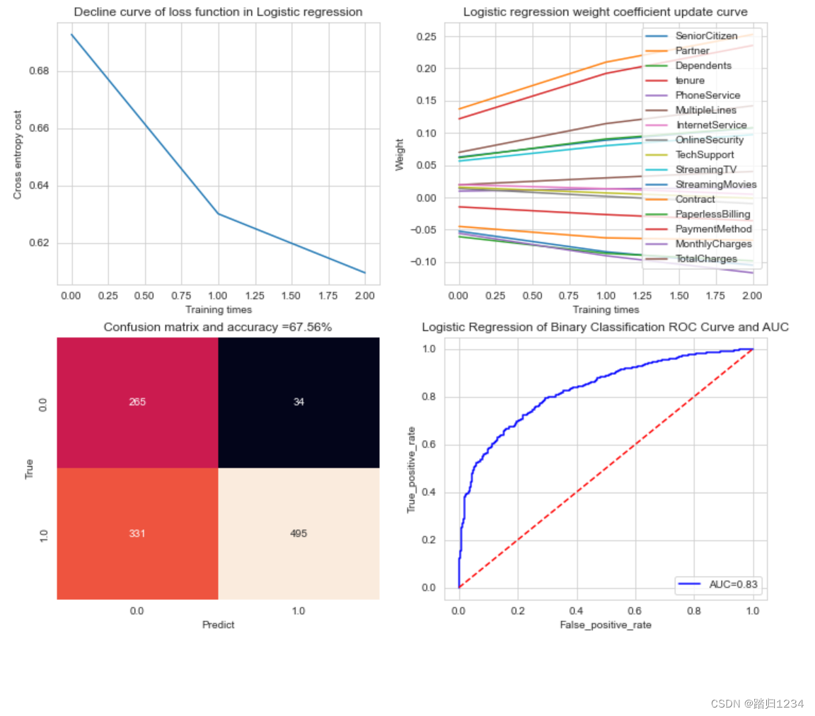
运行结果
可视化,拟合效果不太好
参考资料
网易版 吴恩达机器学习
吴恩达机器学习 网易
2021机器学习(西瓜书+李航统计学习方法)实践部分 + Python

DAMO开发者矩阵,由阿里巴巴达摩院和中国互联网协会联合发起,致力于探讨最前沿的技术趋势与应用成果,搭建高质量的交流与分享平台,推动技术创新与产业应用链接,围绕“人工智能与新型计算”构建开放共享的开发者生态。
更多推荐
 0
0 0
0- 0


 已为社区贡献2条内容

所有评论(0)