【数据结构】哈希表
哈希表(Hash table)是一个根据关键字值(Key value)而直接进行访问的数据结构。也就是说,它通过把关键字的值映射到表中一个位置来访问记录,使插入、删除和查找的效率增加到 O(1)。
哈希表( H a s h t a b l e Hash\ table Hash table),也叫散列表,是一个根据关键字值( K e y v a l u e Key\ value Key value)而直接进行访问的数据结构。也就是说,它通过把关键字的值映射到表中一个位置来访问记录,使插入、删除和查找的效率增加到 O ( 1 ) O(1) O(1)。这个映射函数叫做哈希函数,存放记录的数组叫做哈希表。
一、哈希的概念
哈希( h a s h hash hash)又称散列,是一种组织数据的方式。从译名来看,有散乱排列的意思。本质就是通过哈希函数把关键字 k e y key key 跟存储位置建立一个映射关系,查找时通过这个哈希函数计算出 k e y key key 存储的位置,进行快速查找。
1. 负载因子
负载因子是衡量哈希表填充程度的核心指标,直接关联数据结构的存储效率与操作性能。其数值由已存元素数量除以哈希表总容量得出,合理控制负载因子能有效平衡空间利用率和操作速度。
假设哈希表中已经映射存储了 N N N 个值,哈希表的大小为 M M M,那么负载因子
α = N M \alpha=\frac{N}{M} α=MN
负载因子( l o a d f a c t o r load\ factor load factor)有些地方也翻译为载荷因子 / / /装载因子等。
| 负载因子 | 哈希冲突的概率 | 空间利用率 |
|---|---|---|
| 越大 | 越高 | 越高 |
| 越小 | 越低 | 越低 |
2. 将关键字转为整数
我们将关键字映射到数组中位置,一般是整数容易做映射计算,如果不是整数,我们要想办法转换成整数。
下面哈希函数部分我们讨论时,如果关键字不是整数,那么我们讨论的 k e y key key 是关键字转换成的整数。
二、哈希函数
一个好的哈希函数应该让 N N N 个关键字被等概率的均匀的散列分布到哈希表的 M M M 个空间中,但是实际中却很难做到,但是我们要尽量往这个方向去考量设计。
1. 基本概念
哈希函数( h a s h f u n c t i o n hash\ function hash function)是指将哈希表中元素的关键值映射为元素存储位置的函数。
假设我们有数据范围是 [ 0 , 9999 ] [0, 9999] [0,9999] 的 N N N 个值,我们要映射到一个 M M M 个空间的数组中。(一般情况下, M ≥ N M\ge N M≥N),这个时候关键值的数据范围比较大(比较分散),使用直接定址法就会非常浪费内存。
那么就要借助哈希函数 h f hf hf,关键字 k e y key key 被放到数组的 h f ( k e y ) hf(key) hf(key) 位置:
| 关键字 | 存储位置 | 映射关系 |
|---|---|---|
| N N N 个 k e y key key | 大小为 M M M 的数组 | h f ( k e y ) hf(key) hf(key) 就是存储位置的下标 |
注意: h f ( k e y ) hf(key) hf(key) 计算出的值必须在 [ 0 , M ) [0, M) [0,M) 之间。
2. 直接定址法
当关键字( k e y key key)的范围比较集中时,直接定址法就是非常简单高效的方法。
计数排序就是采用哈希算法中的直接定址法,根据计算关键字的值来作为存储位置:
| 关键字( k e y key key) | 存储位置 | 映射关系 |
|---|---|---|
| [ 0 , 99 ] [0,99] [0,99] | 大小为 100 100 100 的数组 | 每个 k e y key key 的 值 就是存储位置的下标 |
| [ a , z ] [a,z] [a,z] | 大小为 26 26 26 的数组 | 每个 k e y key key 的 值的ASCII码-a 就是存储位置的下标 |
也就是说直接定址法本质就是用关键字( k e y key key)计算出一个绝对位置或者相对位置。
直接定址法的缺点也非常明显:当关键字的范围比较分散时,就很浪费内存甚至内存不够用。
3. 除法散列法 / 除留余数法(重点)
除法散列法也叫做除留余数法,顾名思义,假设哈希表的大小为 M M M,那么通过 k e y key key 除以 M M M 的余数作为映射位置的下标。
也就是哈希函数为: h ( k e y ) = k e y % M h(key) = key\ \%\ M h(key)=key % M
当使用除法散列法时,要尽量避免 M M M 为某些值,如 2 2 2 的幂, 10 10 10 的幂等。
- 如果是 2 x 2^x 2x,那么 k e y % 2 x key\ \%\ 2^x key % 2x 本质相当于保留 k e y key key 的二进制后 x x x 位,那么后 x x x 位相同的值,计算出的哈希值都是一样的,就冲突了。
| 关键字 | M M M ( x = 4 ) (x=4) (x=4) | M M M 的二进制后 4 4 4 位 | 哈希值 h ( k ) = k % M h(k)=k\ \%\ M h(k)=k % M |
|---|---|---|---|
| k 1 = 63 k_1=63 k1=63 | 16 16 16 ( 2 4 ) (2^4) (24) | 1111 1111 1111 | 15 15 15 |
| k 2 = 31 k_2=31 k2=31 | 16 16 16 ( 2 4 ) (2^4) (24) | 1111 1111 1111 | 15 15 15 |
- 如果是 1 0 x 10^x 10x,就更明显了,保留的都是 10 10 10 进值的后 x x x 位。
| 关键字 | M M M ( x = 2 ) (x=2) (x=2) | M M M 的十进制后 2 2 2 位 | 哈希值 h ( k ) = k % M h(k)=k\ \%\ M h(k)=k % M |
|---|---|---|---|
| k 1 = 112 k_1=112 k1=112 | 100 100 100 ( 1 0 2 ) (10^2) (102) | 12 12 12 | 12 12 12 |
| k 2 = 12312 k_2=12312 k2=12312 | 100 100 100 ( 1 0 2 ) (10^2) (102) | 12 12 12 | 12 12 12 |
因此,当使用除法散列法时,建议 M M M 取不太接近 2 2 2 的整数次幂的一个质数(素数)。
4. 乘法散列法(了解)
乘法散列法对哈希表大小 M M M 没有要求,他的大致思路分为两步:
【第一步】用关键字 k e y key key 乘上常数 A A A ( 0 < A < 1 ) (0<A<1) (0<A<1),并抽取出 k e y × A key\times A key×A 的小数部分。
【第二步】再用 M M M 乘以 k × A k\times A k×A 的小数部分,再向下取整。
也就是哈希函数为:
h ( k e y ) = ⌊ M × [ ( A × k e y ) % 1.0 ] ⌋ , A ∈ ( 0 , 1 ) h(key) = \lfloor M\times [(A\times key)\ \%\ 1.0]\rfloor,A\in(0,1) h(key)=⌊M×[(A×key) % 1.0]⌋,A∈(0,1)
这里最重要的是 A A A 的值应该如何设定, K n u t h Knuth Knuth 认为
A = ( 5 − 1 ) 2 ≈ 0.6180339887 … ( 黄金分割点 ) A = \frac{(\sqrt{5} − 1)}{2} \approx 0.6180339887…(黄金分割点) A=2(5−1)≈0.6180339887…(黄金分割点)
比较好。
乘法散列法对哈希表大小 M M M 是没有要求的,比如:
| M M M | k e y key key | A A A | M × [ ( A × k e y ) % 1.0 ] M\times [(A\times key)\ \%\ 1.0] M×[(A×key) % 1.0] | h ( k e y ) h(key) h(key) |
|---|---|---|---|---|
| 1024 1024 1024 | 1234 1234 1234 | 0.6180339887 0.6180339887 0.6180339887 | 669.6366651392 669.6366651392 669.6366651392 | h ( 1234 ) = 669 h(1234)=669 h(1234)=669 |
5. 全域散列法(了解)
如果存在一个恶意的对手,他针对我们提供的散列函数,特意构造出一个发生严重冲突的数据集,
比如,让所有关键字全部落入同一个位置中。这种情况是可以存在的,只要散列函数是公开且确定
的,就可以实现此攻击。
给散列函数增加随机性,攻击者就无法找出确定可以导致最坏情况的数据,这种方法叫做全域散列。
也就是哈希函数为:
h a b ( k e y ) = [ ( a × k e y + b ) % P ] % M h_{ab}(key) = [(a \times key + b)\ \%\ P]\ \%\ M hab(key)=[(a×key+b) % P] % M
P P P 需要选一个足够大的质数, ∀ a , b ∈ Z \forall\ {a,b}\in \mathbb{Z} ∀ a,b∈Z, a ∈ [ 1 , P − 1 ] a\in [1,P-1] a∈[1,P−1], b ∈ [ 0 , P − 1 ] b\in [0,P-1] b∈[0,P−1]。
这些函数构成了一个 P × ( P − 1 ) P\times(P-1) P×(P−1) 组全域散列函数组。
比如:
| P P P | M M M | a a a | b b b | h a b ( k e y ) h_{ab}(key) hab(key) |
|---|---|---|---|---|
| 17 17 17 | 6 6 6 | 3 3 3 | 4 4 4 | h 34 ( 8 ) = 5 h_{34}(8)=5 h34(8)=5 |
注意:每次初始化哈希表时,随机选取全域散列函数组中的一个散列函数使用,后续增删查改都固定使用这个散列函数,否则每次哈希都是随机选一个散列函数,那么插入是一个散列函数,查找又是另一个散列函数,就会导致找不到插入的 k e y key key 了。
三、处理哈希冲突
实践中哈希表一般还是选择除法散列法作为哈希函数,当然哈希表无论选择什么哈希函数也避免不了冲突,那么插入数据时,如何解决冲突呢?主要有两种方法:开放定址法和链地址法。
1. 基本概念
哈希函数存在的一个问题是:两个不同的 k e y key key 可能会映射到同一个位置去,存放和读取数据的时候就会造成冲突和影响,这种问题我们叫做哈希冲突,或者哈希碰撞。
理想情况是找出一个好的哈希函数避免冲突,但是实际场景中,冲突是不可避免的,所以我们尽可能设计出优秀的哈希函数,减少冲突的次数,同时也要去设计出解决冲突的方案。
2. 开放定址法
在开放定址法中所有的元素都放到哈希表里,当一个关键字 k e y key key 用哈希函数计算出的位置冲突了,则按照某种规则找到一个没有存储数据的位置进行存储,开放定址法中负载因子 α \alpha α 一定是小于 1 1 1 的( N < M N<M N<M)。这里的规则有三种:线性探测、二次探测、双重探测。
2.1 线性探测
从发生冲突的位置开始,依次线性向后探测,直到寻找到下一个没有存储数据的位置为止,如果走到哈希表尾,则回绕到哈希表头的位置。
h ( k e y ) = h 0 = k e y % M h(key)=h_0=key\ \%\ M h(key)=h0=key % M, h 0 h_0 h0 位置冲突了,则线性探测公式为:
h c ( k e y , i ) = h i = ( h 0 + i ) % M , i = { 1 , 2 , 3 , … , M − 1 } hc(key,i)=h_i=(h_0+i)\ \%\ M,i=\{1,2,3,…,M-1\} hc(key,i)=hi=(h0+i) % M,i={1,2,3,…,M−1}
因为负载因子 α < 1 \alpha<1 α<1,则最多探测 M − 1 M-1 M−1 次,一定能找到一个存储 k e y key key 的位置。
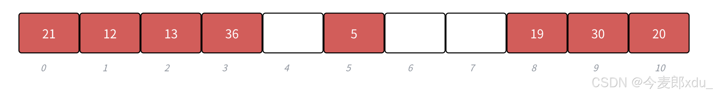
下面演示 { 19,30,5,36,13,20,21,12 } 等这一组值映射到 M = 11 M=11 M=11 的表中:
| k e y key key | 19 19 19 | 30 30 30 | 5 5 5 | 36 36 36 | 13 13 13 | 20 20 20 | 21 21 21 | 12 12 12 |
|---|---|---|---|---|---|---|---|---|
| h 0 h_0 h0 | 8 8 8 | 8 8 8 | 5 5 5 | 3 3 3 | 2 2 2 | 9 9 9 | 10 10 10 | 1 1 1 |
| h 1 h_1 h1 | 9 9 9 | 10 10 10 | 11 11 11 |
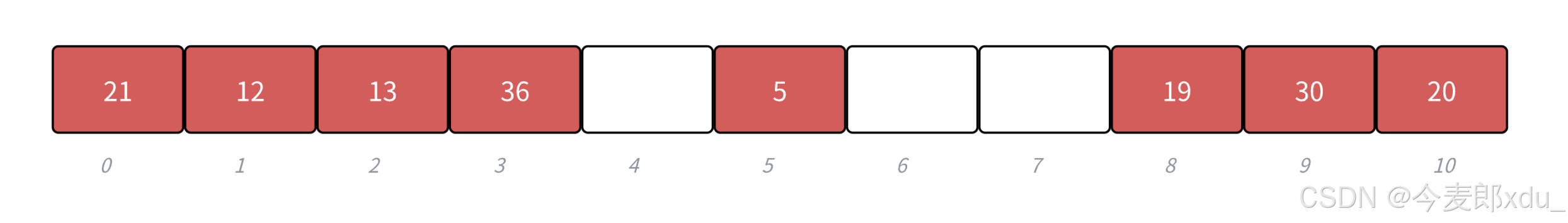
线性探测的比较简单且容易实现,线性探测的问题假设, h 0 h_0 h0 位置连续冲突, h 0 h_0 h0, h 1 h_1 h1, h 2 h_2 h2 位置已经存储数据了,后续映射到 h 0 h_0 h0, h 1 h_1 h1, h 2 h_2 h2, h 3 h_3 h3 的值都会争夺 h 3 h_3 h3 位置,这种现象叫做群集 / / /堆积。下面的二次探测可以一定程度改善这个问题。
2.2 二次探测
从发生冲突的位置开始,依次左右按二次方跳跃式探测,直到寻找到下一个没有存储数据的位置为止,如果往右走到哈希表尾,则回绕到哈希表头的位置;如果往左走到哈希表头,则回绕到哈希表尾的位置。
h ( k e y ) = h 0 = k e y % M h(key) = h_0 = key\ \%\ M h(key)=h0=key % M, h 0 h_0 h0 位置冲突了,则二次探测公式为:
h c ( k e y , i ) = h i = ( h 0 ± i 2 ) % M , i = { 1 , 2 , 3 , . . . , M 2 } hc(key,i) = h_i = (h_0 ± i^2)\ \%\ M, i = \{1, 2, 3, ..., \frac{M}{2}\} hc(key,i)=hi=(h0±i2) % M,i={1,2,3,...,2M}
二次探测当 h i = ( h 0 − i 2 ) % M h_i = (h_0 − i^2)\ \%\ M hi=(h0−i2) % M 时,当 h i < 0 h_i<0 hi<0 时,需要 h i += M h_i \texttt{+=}\ M hi+= M。
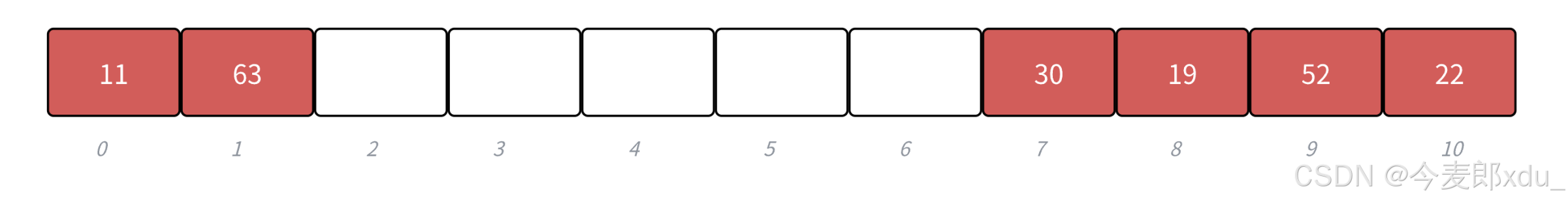
下面演示 { 19,30,52,63,11,22 } 等这一组值映射到 M = 11 M=11 M=11 的表中:
| k e y key key | 19 19 19 | 30 30 30 | 52 52 52 | 63 63 63 | 11 11 11 | 22 22 22 |
|---|---|---|---|---|---|---|
| h 0 h_0 h0 | 8 8 8 | 8 8 8 | 8 8 8 | 8 8 8 | 0 0 0 | 0 0 0 |
| h 1 h_1 h1 | 7 7 7 | 9 9 9 | 7 / 9 7/9 7/9 | 10 10 10 | ||
| h 2 h_2 h2 | 1 1 1 |
2.3 双重散列(了解)
第一个哈希函数计算出的值发生冲突,使用第二个哈希函数计算出一个跟 k e y key key 相关的偏移量值,不断往后探测,直到寻找到下一个没有存储数据的位置为止。其本质也是为了跳跃存取数据,防止堆积。
h 1 ( k e y ) = h 0 = k e y % M h_1(key) = h_0 = key\ \%\ M h1(key)=h0=key % M, h 0 h_0 h0 位置冲突了,则双重探测公式为:
h c ( k e y , i ) = h i = ( h 0 + i × h 2 ( k e y ) ) % M , i = { 1 , 2 , 3 , . . . , M } hc(key,i) = h_i = (h_0 + i \times h_2(key))\ \%\ M,i = \{1, 2, 3,..., M\} hc(key,i)=hi=(h0+i×h2(key)) % M,i={1,2,3,...,M}
要求: h 2 ( k e y ) < M h_2(key) < M h2(key)<M 且 h 2 ( k e y ) h_2(key) h2(key) 和 M M M 互质,有两种简单的取值方法:
-
当 M = 2 x M=2^x M=2x, ∃ x ∈ Z \exists\ x\in \mathbb{Z} ∃ x∈Z 时,从 [ 0 , M − 1 ] [0,M-1] [0,M−1] 中任选一个奇数。
-
当 M M M 为质数时, h 2 ( k e y ) = k e y % ( M − 1 ) + 1 h_2(key) = key\ \%\ (M − 1) + 1 h2(key)=key % (M−1)+1。
注意:保证 h 2 ( k e y ) h_2(key) h2(key) 与 M M M 互质是因为根据固定的偏移量所寻址的所有位置将形成一个群。
如果不互质,则最大公约数 p = g c d ( M , h 2 ( k e y ) ) > 1 p = gcd(M, h_2 (key)) > 1 p=gcd(M,h2(key))>1
那么所能寻址的位置的个数为 M p < M \frac{M}{p} < M pM<M
这使得对于一个关键字( k e y key key)来说无法充分利用整个散列表。
举例来说,若 h 1 ( k e y ) = 1 h_1(key)=1 h1(key)=1, h 2 ( k e y ) = 3 h_2(key)=3 h2(key)=3, M = 12 M=12 M=12:
| h 1 h_1 h1 | h 2 h_2 h2 | h 3 h_3 h3 | h 4 h_4 h4 | ⋅ ⋅ ⋅ ··· ⋅⋅⋅ |
|---|---|---|---|---|
| 1 1 1 | 4 4 4 | 7 7 7 | 10 10 10 | ⋅ ⋅ ⋅ ··· ⋅⋅⋅ |
则所能寻址的位置为 { 1,4,7,10 },即最多能寻址的个数为 12 g c d ( 12 , 3 ) = 4 < 12 \frac{12}{gcd(12, 3)}=4 <12 gcd(12,3)12=4<12,造成空间浪费。
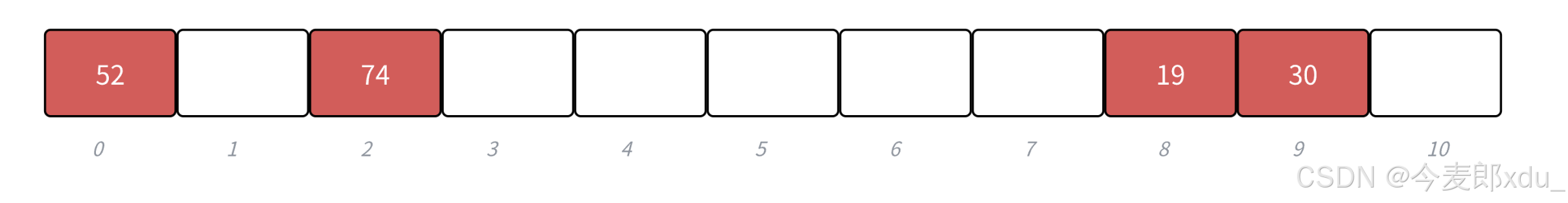
下面演示 { 19,30,52,74 } 等这一组值映射到 M = 11 M=11 M=11 的表中:
因为 M = 11 M=11 M=11 为质数,所以 h 2 ( k e y ) = k e y % 10 + 1 h_2(key) = key\ \%\ 10 + 1 h2(key)=key % 10+1:
| k e y key key | 19 19 19 | 30 30 30 | 52 52 52 | 74 74 74 |
|---|---|---|---|---|
| h 2 ( k e y ) h_2(key) h2(key) | 10 10 10 | 1 1 1 | 3 3 3 | 5 5 5 |
| k e y key key | 19 19 19 | 30 30 30 | 52 52 52 | 74 74 74 |
|---|---|---|---|---|
| h 0 h_0 h0 | 8 8 8 | 8 8 8 | 8 8 8 | 8 8 8 |
| h 1 h_1 h1 | 9 9 9 | 0 0 0 | 2 2 2 |
2.4 实现思路
开放定址法在实践中,始终不如下面要介绍的链地址法(哈希表的主要实现方法)。因为开放定址法解决冲突不管使用哪种方法,占用的都是哈希表中的空间,始终存在互相影响的问题。所以开放定址法,我们简单选择线性探测实现即可。
(1) 哈希表结构
我们用一个顺序表( v e c t o r vector vector)为底层数据结构来封装一个哈希表。这里每个存储值的位置都要加一个状态标识( s t a t e state state),否则删除一些值以后,会影响后面冲突的值的查找。
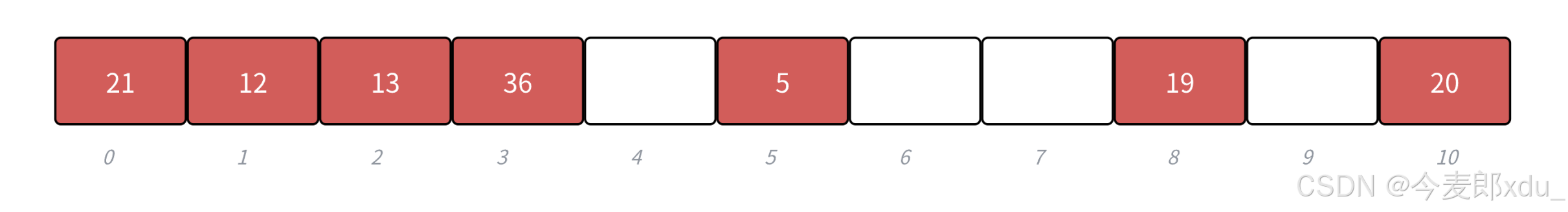
如下图,我们删除 30 30 30,会导致查找 20 20 20 失败:
因为我们是通过开放定址法的线性检测来处理哈希冲突的,因此 20 20 20 从本来应该存储的 9 9 9 下标位置,被迫挪动到了 10 10 10 下标位置:
如果直接查找 20 20 20,那么就会找到 9 9 9 下标位置,但是 9 9 9 为空,结束查找,也就没找到 20 20 20,显然与预期不符:
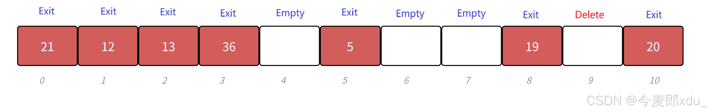
但当我们给每个位置都加一个状态标识 { Exit,Empty,Delete } ,这样删除 30 30 30 的时候就可以不用删除值,而是把状态改为 Delete 即可:
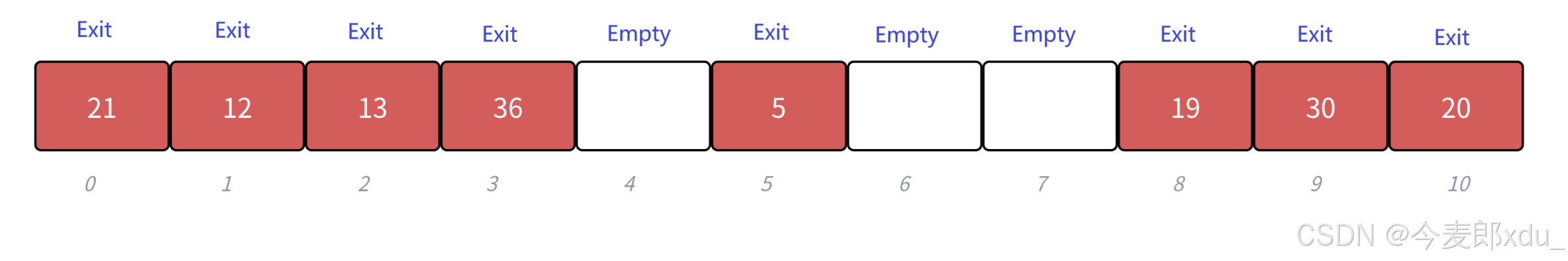
那么查找 20 20 20 时就是遇到 Empty 才能结束,这样就可以找到 20 20 20,符合预期:
// 1.每个存储位的状态标识
enum State
{
	Exist,	// 存在
	Empty,	// 空
	Delete	// 被删除
};

// 2.哈希表的数据类型
template<class K, class V>
struct HashData
{
	pair<K, V> _kv;
	State _st = Empty;
};

// 3.哈希表的基本结构
template<class K, class V>
class HashTable
{
public:
	// ...
private:
	vector<HashData<K, V>> _t;	// 哈希表
	size_t _n = 0;				// 表中存储数据个数
};
(2) 扩容
这里我们把哈希表负载因子 α \alpha α 控制在 0.7 0.7 0.7,当负载因子 α \alpha α 到 0.7 0.7 0.7 以后我们就需要扩容了。和顺序表一样,我们还是按照 2 2 2 倍扩容。
但是同时我们要保持哈希表大小是一个质数,第一个是质数, 2 2 2 倍后就不是质数了,那么如何解决呢?
我们可以使用 S G I SGI SGI 版本的哈希表使用的方法,给了一个近似 2 2 2 倍的质数表,每次去质数表获取扩容后的大小:
inline unsigned long __stl_next_prime(unsigned long n)
{
	// Note: assumes long is at least 32 bits.
	static const int __stl_num_primes = 28;
	static const unsigned long __stl_prime_list[__stl_num_primes] =
	{
	  53, 		  97, 		  193, 		 389, 	    769,
	  1543, 	  3079, 	  6151, 	 12289, 	24593,
	  49157, 	  98317, 	  196613, 	 393241,    786433,
	  1572869, 	  3145739, 	  6291469, 	 12582917,  25165843,
	  50331653,   100663319,  201326611, 402653189, 805306457,
	  1610612741, 3221225473, 4294967291
 	};
 	const unsigned long* first = __stl_prime_list;
	const unsigned long* last = __stl_prime_list + __stl_num_primes;
	const unsigned long* pos = lower_bound(first, last, n);
	return pos == last ? *(last - 1) : *pos;
}
(3) key 不能取模问题
当 k e y key key 是 s t r i n g / D a t e string/Date string/Date 等类型(自定义类型)时, k e y key key 不能取模,那么我们就需要给 H a s h T a b l e HashTable HashTable 增加一个仿函数,这个仿函数支持把 k e y key key 转换成一个可以取模的整型(将关键字转化为整型)。
- 如果 k e y key key 可以转换为整型并且不容易冲突,那么这个仿函数就用默认参数即可。
- 如果这个 k e y key key 不能转换为整型,我们就需要自己实现一个仿函数传给这个参数。
template<class K>
struct HashFunc
{
	size_t operator () (const K& key)
	{
		return (size_t)key;
	}
};

template<class K, class V, class Hash = HashFunc<K>>	// 默认参数强转为 unsigned int
class HashTable
{ // ... };
实现这个仿函数的要求就是尽量让 k e y key key 的每个值都参与到计算中,让不同的 k e y key key 转换出的整型值不同。
但是如果像 s t r i n g string string 这样的自定义类型做哈希表的 k e y key key 非常常见,我们就可以把 s t r i n g string string 特化一下:
template<>
struct HashFunc<string>
{
	size_t operator () (const string& s)
	{
		size_t hash = 0;
		for(auto ch : s)
		{
			hash *= 131;
			hash += ch;
		}
		return hash;
	}
};
2.5 完整代码实现
namespace open_address
{
	enum State
	{
		Exist,
		Empty,
		Delete
	};

	template<class K, class V>
	struct HashData
	{
		pair<K, V> _kv;
		State _st = Empty;
	};

	template<class K, class V, class Hash = HashFunc<K>>
	class HashTable
	{
		Hash hash;

		inline unsigned long __stl_next_prime(unsigned long n)
		{
			// Note: assumes long is at least 32 bits.
			static const int __stl_num_primes = 28;
			static const unsigned long __stl_prime_list[__stl_num_primes] =
			{
			  53, 		  97, 		  193, 		 389, 	    769,
			  1543, 	  3079, 	  6151, 	 12289, 	24593,
			  49157, 	  98317, 	  196613, 	 393241,    786433,
			  1572869, 	  3145739, 	  6291469, 	 12582917,  25165843,
			  50331653,   100663319,  201326611, 402653189, 805306457,
			  1610612741, 3221225473, 4294967291
			};
			const unsigned long* first = __stl_prime_list;
			const unsigned long* last = __stl_prime_list + __stl_num_primes;
			const unsigned long* pos = lower_bound(first, last, n);
			return pos == last ? *(last - 1) : *pos;
		}
	public:
		HashTable()
			:_t(__stl_next_prime(0))
			, _n(0)
		{}

		bool insert(const pair<K, V>& kv)
		{
			if (find(kv.first))
			{
				return false;
			}
			// 如果负载因子 >= 0.7,就扩容
			if (_n * 1.0 / _t.size() >= 0.7)
			{
				HashTable<K, V, Hash> newht;
				newht._t.resize(__stl_next_prime((unsigned long)_t.size() + 1));
				// 将旧表的数据映射到新表
				for (auto& i : _t)
				{
					if (i._st == Exist)
					{
						newht.insert(i._kv);
					}
				}
				_t.swap(newht._t);
			}
			size_t h0 = hash(kv.first) % _t.size();
			size_t hi = h0;
			size_t i = 1;
			while (_t[hi]._st == Exist)
			{
				// 线性探测
				hi = (h0 + i) % _t.size();
				++i;
			}
			_t[hi]._kv = kv;
			_t[hi]._st = Exist;
			++_n;
			return true;
		}

		HashData<K, V>* find(const K& key)
		{
			size_t h0 = hash(key) % _t.size();
			size_t hi = h0;
			size_t i = 1;
			while (_t[hi]._st != Empty)
			{
				if (_t[hi]._st == Exist && _t[hi]._kv.first == key)
				{
					return &_t[hi];
				}
				// 线性探测
				hi = (h0 + i) % _t.size();
				++i;
			}
			return nullptr;
		}

		bool erase(const K& key)
		{
			HashData<K, V>* ret = find(key);
			if (ret)
			{
				ret->_st = Delete;
				return true;
			}
			else
			{
				return false;
			}
		}

		size_t size() const
		{
			return _t.size();
		}
	private:
		vector<HashData<K, V>> _t;
		size_t _n;
	};
}
3. 链地址法(哈希桶)
链地址法中所有的数据不再直接存储在哈希表中,每个存储位存储一个指针,当一个关键字 k e y key key 用哈希函数计算出的位置冲突,就把这些冲突的数据链接成一个链表,挂在哈希表这个位置的下面。链地址法也叫做拉链法或者哈希桶。
3.1 哈希桶的结构
可以将 v e c t o r vector vector 看作一个指针数组,每一个存储位都存储一个结点,依次指向上一个冲突的结点,从而形成一条链表,所有的整体就表示成了一个新的数据结构 —— 哈希桶:
// 1.哈希表中存储的是结点
template<class K, class V>
struct HashNode
{
	pair<K, V>& _kv;
	HashNode<K, V>* _next;

	HashNode(const pair<K, V>& kv)
		:_kv(kv)
		, _next(nullptr)
	{}
};

// 2.哈希桶的基本结构
template<class K, class V, class Hash = HashFunc<K>>
class HashTable
{
	typedef HashNode<K, V> node;
public:
	// ...
private:
	vector<node*> _t;
	size_t _n;
};
3.2 解决冲突的思路
哈希表中每一位都存储一个结点:
- 当没有数据映射这个位置时,这个结点为空。
- 当有多个数据映射到这个位置时,这些冲突的数据的结点链接成一个链表,挂在哈希表这个位置的下面。
下面演示 { 19,30,5,36,13,20,21,12,24,96 } 等这一组值映射到 M = 11 M=11 M=11 的表中:
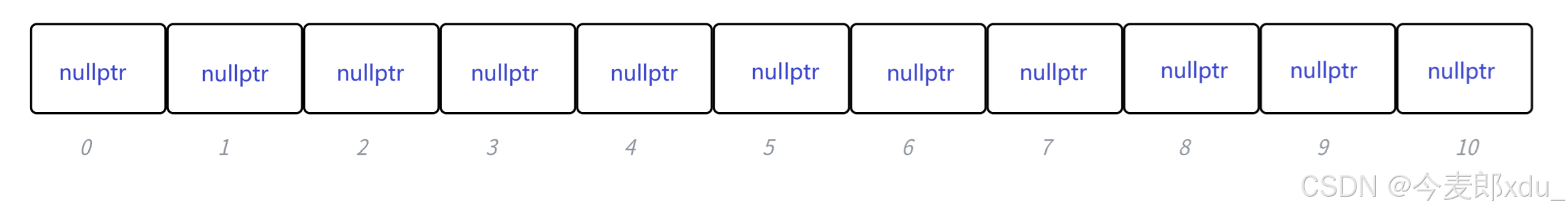
因此哈希函数为 h ( k e y ) = k e y % 11 h(key)=key\ \%\ 11 h(key)=key % 11:
| k e y key key | 19 19 19 | 30 30 30 | 5 5 5 | 36 36 36 | 13 13 13 | 20 20 20 | 21 21 21 | 12 12 12 | 24 24 24 | 96 96 96 |
|---|---|---|---|---|---|---|---|---|---|---|
| h ( k e y ) h(key) h(key) | 8 \color{black}8 8 | 8 \color{red}8 8 | 5 \color{black}5 5 | 3 \color{black}3 3 | 2 \color{black}2 2 | 9 \color{black}9 9 | 10 \color{black}10 10 | 1 \color{black}1 1 | 2 \color{red}2 2 | 8 \color{blue}8 8 |
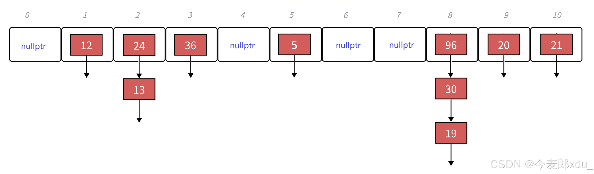
其中,结点插入时相当于链表的头插,每个结点还要指向上一个冲突的结点,这样就能够通过遍历所有冲突值构成的链表找到想要寻找的值了。
极端场景:很容易想到在极端场景下,某个桶会特别长,甚至哈希表可能会直接降成单链表。
虽然使用全域散列法可以避免人为针对,但是偶然情况下,某个桶依然可能很长,查找效率会变得很低。
这里在 J a v a 8 Java8 Java8 的 H a s h M a p HashMap HashMap 中,当桶的长度超过一定阀值( 8 8 8)时就把链表转换成红黑树。但是一般情况下,不断扩容,单个桶很长的场景还是小概率事件。
3.2 扩容
链地址法对负载因子 α \alpha α 没有限制,也就是说 α \alpha α 可以 > 1 >1 >1。
但是负载因子的大小会影响哈希冲突的概率和空间利用率:
| 负载因子 | 哈希冲突的概率 | 空间利用率 |
|---|---|---|
| 越大 | 越高 | 越高 |
| 越小 | 越低 | 越低 |
因此, S T L STL STL 中的 u n o r d e r e d _ x x x unordered\_xxx unordered_xxx 的最大负载因子 α m a x \alpha_{max} αmax 基本控制在 1 1 1,只要 α > 1 \alpha>1 α>1 就扩容,所以我们下面的实现也使用这种方式。
3.3 完整代码实现
namespace hash_bucket
{
	template<class K, class V>
	struct HashNode
	{
		pair<K, V> _kv;
		HashNode<K, V>* _next;

		HashNode(const pair<K, V>& kv)
			:_kv(kv)
			, _next(nullptr)
		{}
	};

	template<class K, class V, class Hash = HashFunc<K>>
	class HashTable
	{
		typedef HashNode<K, V> node;

		Hash hash;

		inline unsigned long __stl_next_prime(unsigned long n)
		{
			// Note: assumes long is at least 32 bits.
			static const int __stl_num_primes = 28;
			static const unsigned long __stl_prime_list[__stl_num_primes] =
			{
			  53, 		  97, 		  193, 		 389, 	    769,
			  1543, 	  3079, 	  6151, 	 12289, 	24593,
			  49157, 	  98317, 	  196613, 	 393241,    786433,
			  1572869, 	  3145739, 	  6291469, 	 12582917,  25165843,
			  50331653,   100663319,  201326611, 402653189, 805306457,
			  1610612741, 3221225473, 4294967291
			};
			const unsigned long* first = __stl_prime_list;
			const unsigned long* last = __stl_prime_list + __stl_num_primes;
			const unsigned long* pos = lower_bound(first, last, n);
			return pos == last ? *(last - 1) : *pos;
		}
	public:
		HashTable()
			:_t(__stl_next_prime(0), nullptr)
			, _n(0)
		{}

		~HashTable()
		{
			for (size_t i = 0; i < _t.size(); i++)
			{
				node* cur = _t[i];
				while (cur)
				{
					node* next = cur->_next;
					delete cur;
					cur = next;
				}
				_t[i] = nullptr;
			}
		}

		bool insert(const pair<K, V>& kv)
		{
			// 扩容
			if (_n == _t.size())
			{
				vector<node*> newtable(__stl_next_prime((unsigned long)_t.size() + 1), nullptr);

				for (size_t i = 0; i < _t.size(); i++)
				{
					node* cur = _t[i];
					while (cur)
					{
						node* next = cur->_next;
						size_t hi = hash(cur->_kv.first) % newtable.size();

						// 将旧表结点头插到新表
						cur->_next = newtable[hi];
						newtable[hi] = cur;

						cur = next;
					}
					_t[i] = nullptr;
				}

				_t.swap(newtable);
			}

			size_t hi = hash(kv.first) % _t.size();
			node* newnode = new node(kv);

			// 头插
			newnode->_next = _t[hi];
			_t[hi] = newnode;
			++_n;

			return true;
		}

		node* find(const K& key)
		{
			size_t hi = hash(key) % _t.size();

			node * cur = _t[hi];
			while (cur)
			{
				if (hash(cur->_kv.first) == hash(key))
				{
					return cur;
				}
				cur = cur->_next;
			}

			return nullptr;
		}

		bool erase(const K& key)
		{
			size_t hi = hash(key) % _t.size();

			node* prev = nullptr;
			node* cur = _t[hi];
			while (cur)
			{
				if (hash(cur->_kv.first) == hash(key))
				{
					if (prev == nullptr)
					{
						// 删除头结点
						_t[hi] = cur->_next;
					}
					else
					{
						// 删除中间结点
						prev->_next = cur->_next;
					}
					delete cur;
					--_n;

					return true;
				}
				else
				{
					prev = cur;
					cur = cur->_next;
				}
			}

			return false;
		}

		size_t size() const
		{
			return _t.size();
		}
	private:
		vector<node*> _t;
		size_t _n;
	};
}
四、hashtable 的模拟实现
1. STL 中的哈希表源码
S G I − S T L 30 SGI-STL\ 30 SGI−STL 30 版本是 C C C++ 11 11 11 之前的 S T L STL STL 版本,因为这个容器是 C C C++ 11 11 11 之后才更新的。 S G I − S T L 30 SGI-STL\ 30 SGI−STL 30 实现了哈希表结构,但是是作为非标准(非标准是指非 C C C++ 标准规定必须实现的)出现的,源码在在头文件 s t l _ h a s h t a b l e . h stl\_hashtable.h stl_hashtable.h 中。
s t l _ h a s h t a b l e . h stl\_hashtable.h stl_hashtable.h:
// stl_hashtable.h
template <class Value, class Key, class HashFcn, class ExtractKey, class EqualKey, class Alloc>
class hashtable {
public:
	typedef Key key_type;
	typedef Value value_type;
	typedef HashFcn hasher;
	typedef EqualKey key_equal;
private:
	hasher hash;
	key_equal equals;
	ExtractKey get_key;
	typedef __hashtable_node<Value> node;
	vector<node*,Alloc> buckets;
	size_type num_elements;
public:
	typedef __hashtable_iterator<Value, Key, HashFcn, ExtractKey, EqualKey, Alloc> iterator;
	pair<iterator, bool> insert_unique(const value_type& obj);
	const_iterator find(const key_type& key) const;
};

template <class Value>
struct __hashtable_node
{
	__hashtable_node* next;
	Value val;
};
通过模板的按需实例化,一个 h a s h t a b l e hashtable hashtable 既可以实现实现 k e y key key 搜索场景的 h a s h _ s e t hash\_set hash_set( u n o r d e r e d _ s e t unordered\_set unordered_set),也可以实现 k e y / v a l u e key/value key/value 搜索场景的 h a s h _ m a p hash\_map hash_map( u n o r d e r e d _ m a p unordered\_map unordered_map):
-
h a s h _ s e t hash\_set hash_set 实例化 h a s h t a b l e hashtable hashtable 时第二个模板参数给的是
key。 -
h a s h _ m a p hash\_map hash_map 实例化 h a s h t a b l e hashtable hashtable 时第二个模板参数给的是
pair<const key, value>。
这样就可以只用一个模板 h a s h t a b l e hashtable hashtable 实现两种不同的容器 h a s h _ s e t / h a s h _ m a p hash\_set/hash\_map hash_set/hash_map,这也体现出了泛型编程的优势。
2. 哈希表的迭代器
2.1 iterator 源码
template <class Value, class Key, class HashFcn, class ExtractKey, class EqualKey, class Alloc>
struct __hashtable_iterator
{
	typedef hashtable<Value, Key, HashFcn, ExtractKey, EqualKey, Alloc> hashtable;
	typedef __hashtable_iterator<Value, Key, HashFcn, ExtractKey, EqualKey, Alloc> iterator;
	typedef __hashtable_const_iterator<Value, Key, HashFcn, ExtractKey, EqualKey, Alloc> const_iterator;
	typedef __hashtable_node<Value> node;
	typedef forward_iterator_tag iterator_category;
	typedef Value value_type;
	node* cur;
	hashtable* ht;
	__hashtable_iterator(node* n, hashtable* tab)
		: cur(n)
		, ht(tab)
	{}
	__hashtable_iterator()
	{}
	reference operator*() const
	{
		return cur->val;
	}
	#ifndef __SGI_STL_NO_ARROW_OPERATOR
	pointer operator->() const { return &(operator*()); }
	#endif /* __SGI_STL_NO_ARROW_OPERATOR */
	iterator& operator++();
	iterator operator++(int);
	bool operator==(const iterator& it) const
	{
		return cur == it.cur;
	}
	bool operator!=(const iterator& it) const
	{
		return cur != it.cur;
	}
};

template <class V, class K, class HF, class ExK, class EqK, class A>
__hashtable_iterator<V, K, HF, ExK, EqK, A>& __hashtable_iterator<V, K, HF, ExK, EqK, A>::operator++()
{
	const node* old = cur;
	cur = cur->next;
	if (!cur)
	{
		size_type bucket = ht->bkt_num(old->val);
		while (!cur && ++bucket < ht->buckets.size())
		{
			cur = ht->buckets[bucket];
		}
	}
	return *this;
}
2.2 实现思路
i t e r a t o r iterator iterator 实现的大框架跟 l i s t list list 的 i t e r a t o r iterator iterator 思路是一致的,用一个类型封装结点的指针,再通过重载运算符实现,迭代器像指针一样访问的行为,要注意的是哈希表的迭代器是单向迭代器( f o r w a r d i t e r a t o r forward\ iterator forward iterator)。
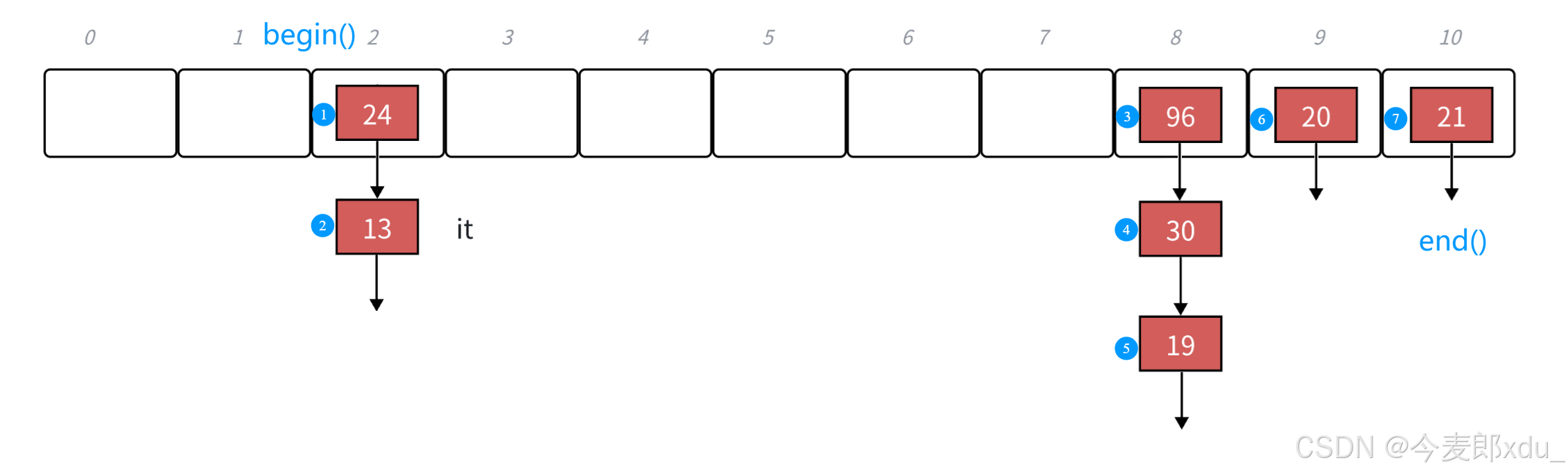
b e g i n ( ) begin() begin():返回第一个桶中第一个结点指针构造的迭代器。
iterator begin()
{
	if(_n == 0)
		return end();
	for(size_t i = 0; i < _t.size(); ++i)
	{
		node* cur = _t[i];
		while(cur)
		{
			return iterator(cur, this);
		}
	}
	return end();
}
e n d ( ) end() end():返回迭代器可以用 n u l l p t r \color{blue}nullptr nullptr 表示。
iterator end()
{
	return iterator(nullptr, this);
}
这里的难点是 o p e r a t o r operator operator++ 的实现。(和 l i s t list list 最大的不同)
i t e r a t o r iterator iterator 中有一个指向结点的指针:
-
如果当前桶下面还有结点,则结点的指针指向下一个结点即可。
-
如果当前桶走完了,则需要想办法计算找到下一个桶。
这里的难点是反而是结构设计的问题,参考上面的源码,我们可以看到 i t e r a t o r iterator iterator 中除了有结点的指针,还有哈希表对象的指针:
struct iterator
{
	node* _node;			// 结点的指针
	const hashtable* _ht;	// 哈希表对象的指针

	// 这里_ht要给const权限是因为要适配cbegin/cend(const函数)返回的this指针
	hash_iterator(node* node, const hashtable* ht)
		:_node(node)
		, _ht(ht)
	{}
}
这样当前桶走完了,要计算下一个桶就相对容易多了,用 k e y key key 值计算出当前桶位置,依次往后找下一个不为 n u l l p t r nullptr nullptr 的桶即可(遍历哈希表)。
3. 哈希封装
之前的哈希桶的模拟实现直接使用的是 p a i r pair pair 类型作为数据类型,这对于 u n o r d e r e d _ s e t unordered\_set unordered_set 容器是不适用的,为了能适配 u n o r d e r e d _ m a p unordered\_map unordered_map 和 u n o r e d e r _ s e t unoreder\_set unoreder_set 两种容器的底层使用,这里统一进行了泛型修改:使用 T T T 作为数据的类型,以及对迭代器也进行实现和封装。这样 u n o r d e r e d _ m a p unordered\_map unordered_map 和 u n o r e d e r _ s e t unoreder\_set unoreder_set 的模拟实现就可以直接使用这个泛型版本的哈希桶。
进行泛型修改和迭代器封装后的 h a s h t a b l e . h hashtable.h hashtable.h:
#pragma once
#include<iostream>
#include<vector>
#include<unordered_set>
#include<unordered_map>

using namespace std;

namespace ybc
{
	template<class K>
	struct hash
	{
		size_t operator () (const K& key)
		{
			return (size_t)key;
		}
	};

	// 特化
	template<>
	struct hash<string>
	{
		size_t operator() (const string& s)
		{
			size_t hash = 0;
			for (auto ch : s)
			{
				hash *= 131;
				hash += ch;
			}
			return hash;
		}
	};

	template<class T>
	struct hash_node
	{
		T _data;
		hash_node<T>* _next;

		hash_node(const T& data)
			:_data(data)
			, _next(nullptr)
		{}
	};

	// 前置声明
	template<class K, class T, class KeyOfT, class Hash>
	class hashtable;

	template<class K, class T, class Ptr, class Ref, class KeyOfT, class Hash>
	struct hash_iterator
	{
		typedef hash_node<T> node;
		typedef hashtable<K, T, KeyOfT, Hash> hashtable;
		typedef hash_iterator<K, T, Ptr, Ref, KeyOfT, Hash> self;

		node* _node;			// 当前结点的指针
		const hashtable* _ht;	// 哈希表对象的指针

		KeyOfT kot;
		Hash hash;

		hash_iterator(node* node, const hashtable* ht)
			:_node(node)
			, _ht(ht)
		{}

		Ptr operator->()
		{
			return &_node->_data;
		}

		Ref operator*()
		{
			return _node->_data;
		}

		self& operator ++ ()
		{
			if (_node->_next)
			{
				// 当前桶还有结点
				_node = _node->_next;
				return *this;
			}
			else
			{
				// 当前桶走完了,寻找下一个桶
				size_t hi = hash(kot(_node->_data)) % _ht->_t.size();
				while (++hi < _ht->_t.size())
				{
					if (_ht->_t[hi])
					{
						_node = _ht->_t[hi];
						return *this;
					}
				}
				_node = nullptr;
				return *this;
			}
		}

		bool operator == (const self& s)
		{
			return _node == s._node;
		}

		bool operator != (const self& s)
		{
			return _node != s._node;
		}
	};

	template<class K, class T, class KeyOfT, class Hash>
	class hashtable
	{
		// 模板类的友元声明要带模板
		template<class K, class T, class Ptr, class Ref, class KeyOfT, class Hash>
		friend struct hash_iterator;

		typedef hash_node<T> node;

		KeyOfT kot;
		Hash hash;
	public:
		typedef hash_iterator<K, T, T*, T&, KeyOfT, Hash> iterator;
		typedef hash_iterator<K, T, const T*, const T&, KeyOfT, Hash> const_iterator;

		iterator begin()
		{
			if (_n == 0)
			{
				return end();
			}
			for (size_t i = 0; i < _t.size(); ++i)
			{
				node* cur = _t[i];
				if (cur)
				{
					return iterator(cur, this);
				}
			}
			return end();
		}

		iterator end()
		{
			return iterator(nullptr, this);
		}

		const_iterator cbegin() const
		{
			if (_n == 0)
			{
				return cend();
			}
			for (size_t i = 0; i < _t.size(); ++i)
			{
				node* cur = _t[i];
				if (cur)
				{
					return const_iterator(cur, this);
				}
			}
			return cend();
		}

		const_iterator cend() const
		{
			return const_iterator(nullptr, this);
		}

		inline unsigned long __stl_next_prime(unsigned long n)
		{
			// Note: assumes long is at least 32 bits.
			static const int __stl_num_primes = 28;
			static const unsigned long __stl_prime_list[__stl_num_primes] =
			{
			  53, 		  97, 		  193, 		 389, 	    769,
			  1543, 	  3079, 	  6151, 	 12289, 	24593,
			  49157, 	  98317, 	  196613, 	 393241,    786433,
			  1572869, 	  3145739, 	  6291469, 	 12582917,  25165843,
			  50331653,   100663319,  201326611, 402653189, 805306457,
			  1610612741, 3221225473, 4294967291
			};
			const unsigned long* first = __stl_prime_list;
			const unsigned long* last = __stl_prime_list + __stl_num_primes;
			const unsigned long* pos = lower_bound(first, last, n);
			return pos == last ? *(last - 1) : *pos;
		}

		hashtable()
			:_t(__stl_next_prime(0), nullptr)
			, _n(0)
		{}

		~hashtable()
		{
			for (size_t i = 0; i < _t.size(); ++i)
			{
				node* cur = _t[i];
				while (cur)
				{
					node* next = cur->_next;
					delete cur;
					cur = next;
				}
				_t[i] = nullptr;
			}
		}

		pair<iterator, bool> insert(const T& data)
		{
			iterator it = find(kot(data));
			if (it != end())
			{
				return make_pair(it, false);
			}
			if (_n == _t.size())
			{
				vector<node*> newtable(__stl_next_prime((unsigned long)_t.size() + 1), nullptr);
				for (size_t i = 0; i < _t.size(); ++i)
				{
					node* cur = _t[i];
					while (cur)
					{
						node* next = cur->_next;
						size_t hi = hash(kot(cur->_data)) % newtable.size();

						cur->_next = newtable[hi];
						newtable[hi] = cur;
						cur = next;
					}
					_t[i] = nullptr;
				}
				_t.swap(newtable);
			}

			size_t hi = hash(kot(data)) % _t.size();
			node* newnode = new node(data);
			newnode->_next = _t[hi];
			_t[hi] = newnode;
			++_n;

			return make_pair(iterator(newnode, this), true);
		}

		iterator find(const K& key)
		{
			size_t hi = hash(key) % _t.size();
			node* cur = _t[hi];
			while (cur)
			{
				if (kot(cur->_data) == key)
				{
					return iterator(cur, this);
				}
				cur = cur->_next;
			}
			return end();
		}

		bool erase(const K& key)
		{
			size_t hi = hash(key) % _t.size();
			node* prev = nullptr;
			node* cur = _t[hi];
			while (cur)
			{
				if (kot(cur->_data) == key)
				{
					if (prev == nullptr)
					{
						_t[hi] = cur->_next;
					}
					else
					{
						prev->_next = cur->_next;
					}
					delete cur;
					--_n;
					return true;
				}
				else
				{
					prev = cur;
					cur = cur->_next;
				}
			}
			return false;
		}
	private:
		vector<node*> _t;
		size_t _n;
	};
}
总结
H a s h Hash Hash 是散列的意思,但一般音译成哈希。这里的哈希表就是利用哈希算法,把输入数据通过哈希函数转换为哈希值,哈希值就作为数组的地址来直接存储数据,这样能使增删改查的效率提升至 O ( 1 ) O(1) O(1)。
而这种转换是一种压缩映射,也就是说必然存在哈希冲突,不可能从哈希值来确定唯一的输入值。
在 S G I − S T L 30 SGI-STL\ 30 SGI−STL 30 版本中,非标准容器 h a s h _ s e t hash\_set hash_set 和 h a s h _ m a p hash\_map hash_map 的底层结构使用的数据结构是 h a s h t a b l e hashtable hashtable,其是用哈希桶实现的,哈希桶是用链地址法处理哈希冲突的哈希表。
u n o r d e r e d _ s e t unordered\_set unordered_set 和 u n o r d e r e d _ m a p unordered\_map unordered_map 是在 C C C++ 11 11 11 之后才被列入标准库的,其底层结构依然为哈希桶。

DAMO开发者矩阵,由阿里巴巴达摩院和中国互联网协会联合发起,致力于探讨最前沿的技术趋势与应用成果,搭建高质量的交流与分享平台,推动技术创新与产业应用链接,围绕“人工智能与新型计算”构建开放共享的开发者生态。
更多推荐


 27
27 0
0- 0


 已为社区贡献2条内容

所有评论(0)