空域滤波增强

First : imnoise()

 

clc;close all;I = imread('图片2.jpg');subplot(121),imshow(I);title('原始图像');J = imnoise(I,'salt & pepper');subplot(122),imshow(J);title('加入椒盐噪声后的图像')

RESULT

空域滤波过程

Spocess

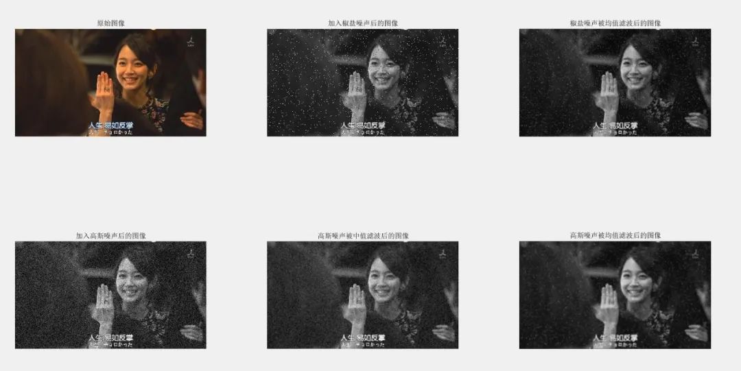
clc;close all;I = imread('图片2.jpg');subplot(231),imshow(I);title('原始图像');I = rgb2gray(I);J = imnoise(I,'salt & pepper',0.03);% 加均值为0，方差为0.03的椒盐噪声subplot(232),imshow(J);title('加入椒盐噪声后的图像')K = filter2(fspecial('average',3),J)/255; % 进行“相关”计算% 注：fspecial()函数可产生 ‘average’, ‘gaussian’, ‘motion’, ‘sobel’, ‘laplacian’,  ‘log’ , ‘unsharp’ 等多种特殊滤波器subplot(233),imshow(K,[]);title('椒盐噪声被均值滤波后的图像');J2 = imnoise(I,'gaussian',0.03); %% 加均值为0，方差为0.03的高斯噪声subplot(234),imshow(J2);title('加入高斯噪声后的图像');K2 = medfilt2(J2); % 图像滤波处理(中值滤波函数)subplot(235),imshow(K2,[]);title('高斯噪声被中值滤波后的图像');K3 = filter2(fspecial('average',5),J)/255; % 进行“相关”计算subplot(236),imshow(K3,[]);title('高斯噪声被均值滤波后的图像');

RESULT

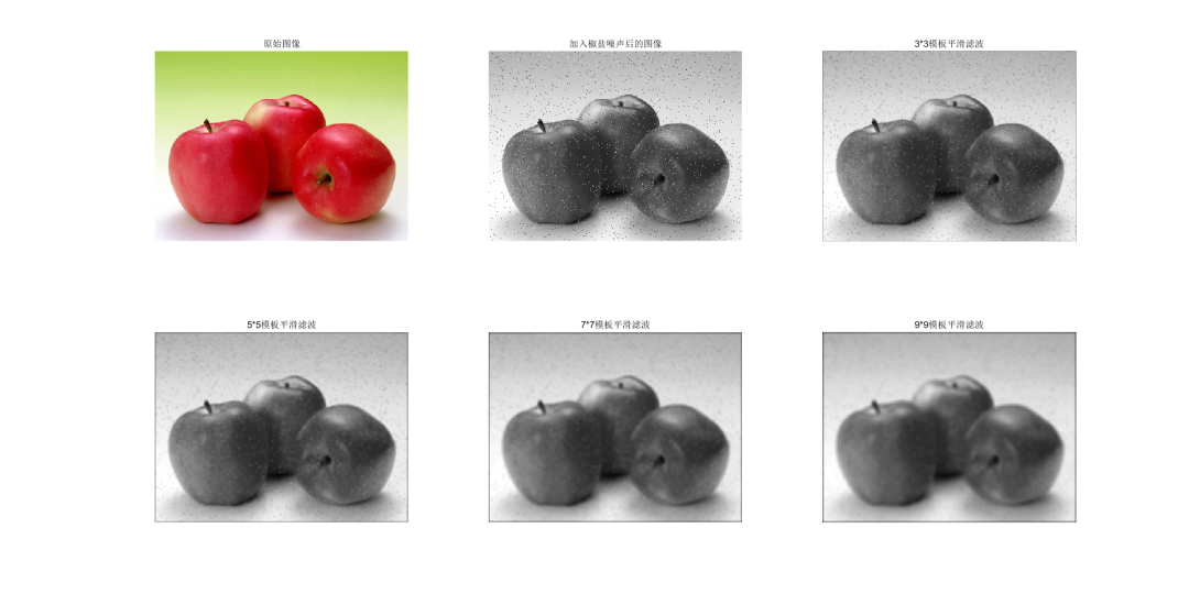
通过不同的滤波窗口对图像进行平滑滤波处理

filter2(fspecial('average',n),I)

clc;close all;I = imread('图片4.jpg');subplot(231),imshow(I);title('原始图像');I = rgb2gray(I);J = imnoise(I,'salt & pepper',0.02); % 加均值为0，方差为0.02的椒盐噪声subplot(232),imshow(J);title('加入椒盐噪声后的图像')K1 = filter2(fspecial('average',3),J); % 进行3*3模板平滑滤波K2 = filter2(fspecial('average',5),J); % 进行5*5模板平滑滤波K3 = filter2(fspecial('average',7),J); % 进行7*7模板平滑滤波K4 = filter2(fspecial('average',9),J); % 进行9*9模板平滑滤波subplot(233),imshow(uint8(K1));title('3*3模板平滑滤波');subplot(234),imshow(uint8(K2));title('5*5模板平滑滤波');subplot(235),imshow(uint8(K3));title('7*7模板平滑滤波');subplot(236),imshow(uint8(K4));title('9*9模板平滑滤波');

RESULT

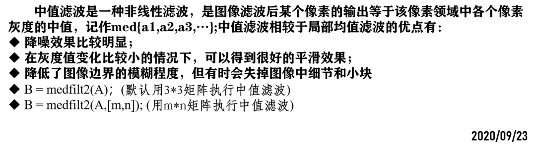
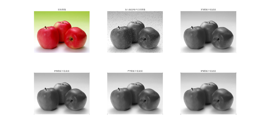
中值滤波

Median Filtering

clc;close all;I = imread('图片4.jpg');subplot(231),imshow(I);title('原始图像');I = rgb2gray(I);J = imnoise(I,'salt & pepper',0.02);% 加均值为0，方差为0.02的椒盐噪声subplot(232),imshow(J);title('加入椒盐噪声后的图像')K1 = medfilt2(J);       % 进行3*3模板中值滤波K2 = medfilt2(J,[5,5]); % 进行5*5模板中值滤波K3 = medfilt2(J,[7,7]); % 进行7*7模板中值滤波K4 = medfilt2(J,[9,9]); % 进行9*9模板中值滤波subplot(233),imshow(K1);title('3*3模板中值滤波');subplot(234),imshow(K2);title('5*5模板中值滤波');subplot(235),imshow(K3);title('7*7模板中值滤波');subplot(236),imshow(K4);title('9*9模板中值滤波');

RESULT

利用中值滤波去除图像中的多种噪声

|||

clc;close all;I = imread('图片4.jpg');I = rgb2gray(I);J1 = imnoise(I,'salt & pepper',0.02);% 加均值为0，方差为0.02的椒盐噪声J2 = imnoise(I,'gaussian',0,0.02);   % 加均值为0，方差为0.02的高斯噪声J3 = imnoise(I,'speckle',0.02);      % 加均值为0，方差为0.02的乘性噪声K1 = medfilt2(J1);  % 进行3*3模板对椒盐噪声中值滤波K2 = medfilt2(J2);  % 进行3*3模板对高斯噪声中值滤波K3 = medfilt2(J3);  % 进行3*3模板对乘性噪声中值滤波subplot(231),imshow(J1);title('加入椒盐噪声后的图像')subplot(232),imshow(J2);title('加入高斯噪声后的图像')subplot(233),imshow(J3);title('加入乘性噪声后的图像')subplot(234),imshow(K1);title('3*3模板对椒盐噪声中值滤波');subplot(235),imshow(K2);title('3*3模板对高斯噪声中值滤波');subplot(236),imshow(K3);title('3*3模板对乘性噪声中值滤波');

RESULT

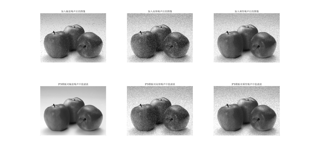
结论：椒盐噪声和中值滤波搞CP

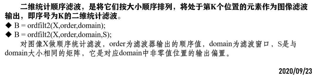
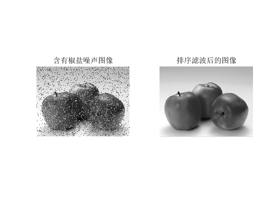
二维统计顺序滤波

GTwo dimensional statistical sequential filtering

clc;close all;I = imread('图片4.jpg');I = rgb2gray(I);I = imnoise(I,'salt & pepper',0.1);% 加均值为0，方差为0.02的椒盐噪声domain = [0 1 1 0;1 1 1 1;1 1 1 1;0 1 1 0];J = ordfilt2(I,6,domain);subplot(121),imshow(I);title('含有椒盐噪声图像');subplot(122),imshow(J);title('排序滤波后的图像');

RESULT

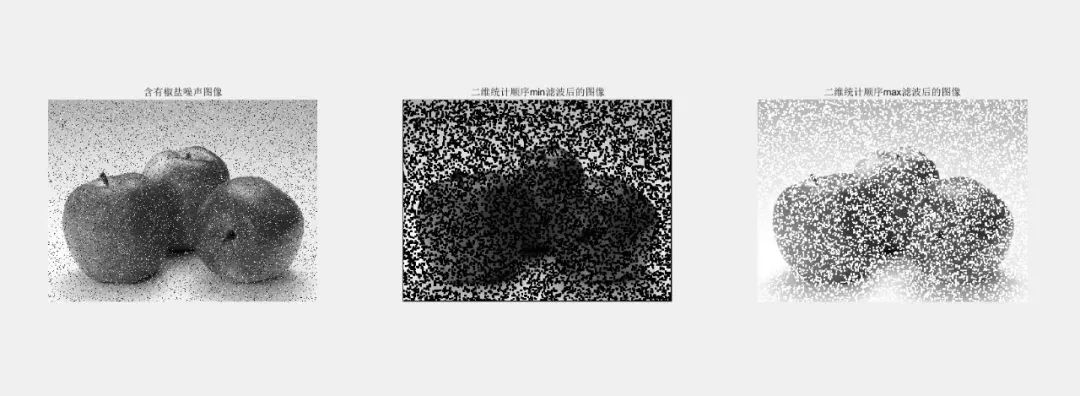
采用最大值和最小值进行滤波增强

GThe maximum and minimum values are used for filtering enhancement

clc;close all;I = imread('图片4.jpg');I = rgb2gray(I);I = imnoise(I,'salt & pepper',0.1);% 加均值为0，方差为0.02的椒盐噪声J1 = ordfilt2(I,1,ones(4));J2 = ordfilt2(I,9,ones(3));subplot(131),imshow(I);title('含有椒盐噪声图像');subplot(132),imshow(J1);title('二维统计顺序min滤波后的图像');subplot(133),imshow(J2);title('二维统计顺序max滤波后的图像');%% 总结% B = ordfilt2(A,5,ones(3,3)) implements a 3-by-3 median filter; % B = ordfilt2(A,1,ones(3,3)) implements a 3-by-3 minimum filter; % B = ordfilt2(A,9,ones(3,3)) implements a 3-by-3 maximum filter.

RESULT

补充：自适应滤波

Adaptive Filtering

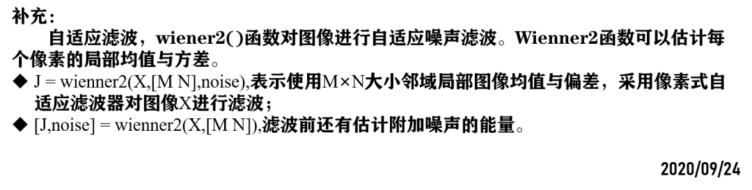
clc;close all;I = imread('图片4.jpg');I = rgb2gray(I);I = imnoise(I,'gaussian',0.1);% 加均值为0，方差为0.02的椒盐噪声[J,noise] = wiener2(I,[5,5]);subplot(121),imshow(I);title('含有高斯噪声图像');subplot(122),imshow(J);title('自适应滤波后的图像');

RESULT

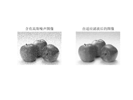
clc;close all;I = imread('图片4.jpg');subplot(231),imshow(I);title('原图');I = rgb2gray(I);I = imnoise(I,'salt & pepper',0.1);% 加均值为0，方差为0.02的椒盐噪声J1 = wiener2(I,[3 3]);% 进行3*3模板自适应滤波 J2 = wiener2(I,[5 5]);% 进行5*5模板自适应滤波J3 = wiener2(I,[7 7]);% 进行7*7模板自适应滤波J4 = wiener2(I,[9 9]);% 进行9*9模板自适应滤波subplot(232),imshow(I);title('含有椒盐噪声图像');subplot(233),imshow(J1);title('3*3模板自适应滤波');subplot(234),imshow(J2);title('5*5模板自适应滤波');subplot(235),imshow(J3);title('7*7模板自适应滤波');subplot(236),imshow(J4);title('9*9模板自适应滤波');

RESULT

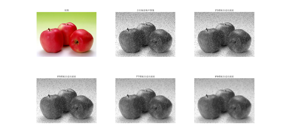
锐化滤波

Sharpen filter

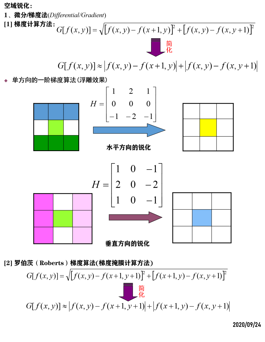
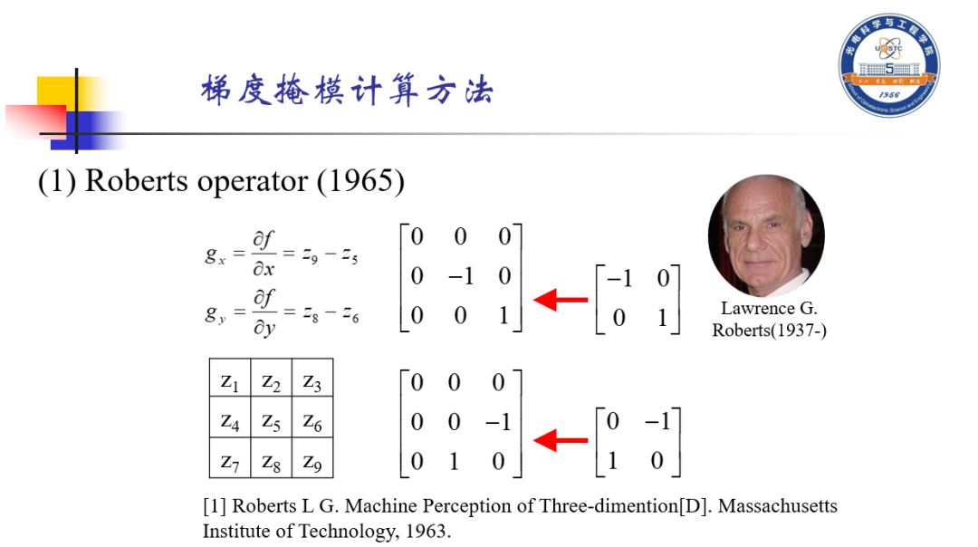
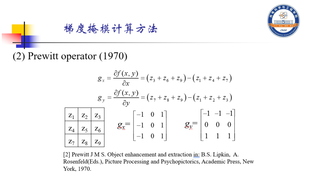
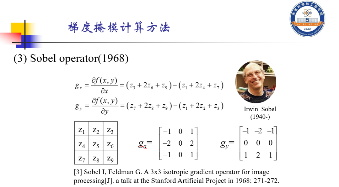
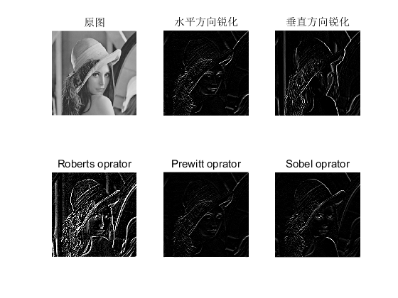
clc;close all;I = imread('图片6.png');figure(2)subplot(231),imshow(I);title('原图');I = rgb2gray(I);H1 = [1 2 1;0 0 0;-1 -2 -1];J1 = imfilter(I,H1); % 水平方向锐化H2 = [1 0 -1;2 0 -2;1 0 -1];J2 = imfilter(I,H2); % 垂直方向锐化H3 = 20*[0 0 0;0 -1 0;0 0 1]; % 放大了一下，太弱了；(这里有点问题，Roberts算子得再想想)% H31 = [1 0;0 -1];H32 = [0 1;-1 0];% H3 = 2*H31 + 3*H32;J3 = imfilter(I,H3); % Roberts opratorH4 = [1 1 1;0 0 0;-1 -1 -1];J4 = imfilter(I,H4); % Prewitt opratorH5 = [-1 -2 -1;0 0 0;1 2 1];J5 = imfilter(I,H5); % Prewitt opratorsubplot(232),imshow(J1);title('水平方向锐化');subplot(233),imshow(J2);title('垂直方向锐化');subplot(234),imshow(J3);title('Roberts oprator');subplot(235),imshow(J4);title('Prewitt oprator');subplot(236),imshow(J5);title('Sobel oprator');

RESULT

%% 说明% 在这里生成Roberts算子的方法不一样，结果存在一定的问题！！！！！clc;close all;I = imread('图片6.png');subplot(131),imshow(I);title('原图');I = rgb2gray(I);BW1 = edge(I,'roberts',0.1); %选择Roberts算子subplot(132),imshow(BW1);title('Roberts算子');hp = fspecial('prewitt'); % 选择Prewitt算子P = imfilter(I,hp);subplot(133),imshow(P);title('Prewitt算子')

RESULT

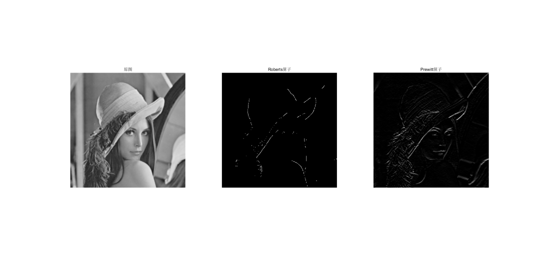
这是干了个啥。。。越做越不明显

搞不懂Roberts算子啊

【等老师讲吧】