融合Transformer与LSTM的时序预测：原理与电力负荷预测实践,10分钟包你上手！！！

2501_93508870

845人浏览 · 2025-10-17 15:26:06

2501_93508870 · 2025-10-17 15:26:06 发布

时间序列预测中，LSTM擅长捕捉局部时序依赖却难及长距关联，Transformer凭自注意力突破长距限制但缺乏时序感知。二者互补成研究热点——融合模型既能借LSTM锚定时序流，又以Transformer挖掘全局关联。

沉迷学习ing

今天带大家通过实操上手项目，讲讲这个热点方向！所涉及到的源码和相关论文感兴趣的dd~

原文资料这里！

1. 时间序列预测基础

时间序列是按时间顺序排列的数据点序列，数学上可表示为 ${x_1, x_2, ..., x_T\}$ ，其中 $x_t \in \mathbb{R}^d$ 表示 $t$ 时刻的 $d$ 维观测值。时间序列预测的核心任务是：给定历史观测值 ${x_1, ..., x_t\}$ ，预测未来值 ${x_{t+1}, ..., x_{t+k}\}$ ，其中 $k$ 为预测步长。

在实际应用中，时间序列通常包含以下成分：

趋势项（Trend）：长期整体变化趋势
季节性（Seasonality）：周期性波动
噪声（Noise）：随机扰动

数学上可表示为： $x_t = T_t + S_t + \epsilon_t$ ，其中 $T_t$ 为趋势项， $S_t$ 为季节项， $\epsilon_t$ 为噪声项。

2. LSTM原理详解

2.1 循环神经网络局限

传统循环神经网络（RNN）存在梯度消失/爆炸问题，难以捕捉长序列依赖。其更新公式为：
$h_t = \sigma(W_{xh}x_t + W_{hh}h_{t-1} + b_h)$
$y_t = W_{hy}h_t + b_y$
其中 $h_t$ 为隐藏状态， $\sigma$ 为激活函数， $W$ 和 $b$ 为可学习参数。当序列较长时，梯度通过时间反向传播会导致梯度指数级衰减或增长。

2.2 LSTM的门控机制

LSTM模型结构

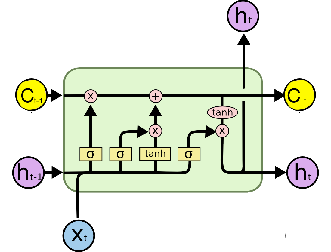
长短期记忆网络（LSTM）通过门控机制解决长序列依赖问题，其核心是细胞状态 $c_t$ 和三个门控单元：

遗忘门（Forget Gate）：决定保留多少历史细胞状态
$f_t = \sigma(W_f \cdot [h_{t-1}, x_t] + b_f) \tag{1}$
输入门（Input Gate）：决定更新哪些信息
$i_t = \sigma(W_i \cdot [h_{t-1}, x_t] + b_i) \tag{2}$
$\tilde{c}_t = \tanh(W_c \cdot [h_{t-1}, x_t] + b_c) \tag{3}$
细胞状态更新：
$c_t = f_t \odot c_{t-1} + i_t \odot \tilde{c}_t \tag{4}$
其中 $\odot$ 表示元素级乘法
输出门（Output Gate）：决定输出信息
$o_t = \sigma(W_o \cdot [h_{t-1}, x_t] + b_o) \tag{5}$
$h_t = o_t \odot \tanh(c_t) \tag{6}$

LSTM通过上述机制有效控制信息的流动和保留，能够捕捉时间序列中的长期依赖关系。

3. Transformer原理详解

3.1 自注意力机制

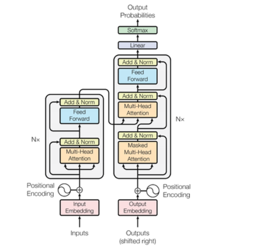
Transformer基于自注意力机制（Self-Attention），能够直接建模序列中任意位置的依赖关系。给定查询（Query） $\in \mathbb{R}^{n \times d_k}$ 、键（Key） $\in \mathbb{R}^{n \times d_k}$ 和值（Value） $\in \mathbb{R}^{n \times d_v}$ ，注意力计算为：

$\text{Attention}(Q, K, V) = \text{softmax}\left(\frac{QK^T}{\sqrt{d_k}}\right)V \tag{7}$

其中 $\sqrt{d_k}$ 为缩放因子，用于防止内积过大导致softmax梯度消失。
Transformer模型原理图

3.2 多头注意力

多头注意力（Multi-Head Attention）通过多个并行的注意力头捕捉不同类型的依赖关系：

$\text{MultiHead}(Q, K, V) = \text{Concat}(\text{head}_1, ..., \text{head}_h)W^O \tag{8}$
$\text{head}_i = \text{Attention}(QW_i^Q, KW_i^K, VW_i^V) \tag{9}$

其中 $h$ 为头数， $W_i^Q \in \mathbb{R}^{d_{\text{model}} \times d_k}$ ， $W_i^K \in \mathbb{R}^{d_{\text{model}} \times d_k}$ ， $W_i^V \in \mathbb{R}^{d_{\text{model}} \times d_v}$ ， $W^O \in \mathbb{R}^{hd_v \times d_{\text{model}}}$ 为可学习参数。

3.3 位置编码

Transformer本身是并行计算的，不包含时序信息，需通过位置编码（Positional Encoding）注入序列位置信息：

$PE_{(pos, 2i)} = \sin\left(\frac{pos}{10000^{2i/d_{\text{model}}}}\right) \tag{10}$
$PE_{(pos, 2i+1)} = \cos\left(\frac{pos}{10000^{2i/d_{\text{model}}}}\right) \tag{11}$

其中 $p os$ 为位置索引， $i$ 为维度索引。

4. 融合Transformer与LSTM的模型设计

融合模型结合LSTM的时序建模能力和Transformer的长距离依赖捕捉能力，架构如下：
融合Transformer与LSTM的模型设计

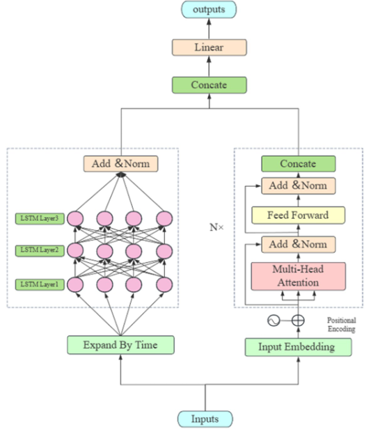
输入层：接收时间序列数据，进行标准化处理
LSTM编码器：提取局部时序特征
$h_t^{\text{LSTM}} = \text{LSTM}(x_t, h_{t-1}^{\text{LSTM}}) \tag{12}$
Transformer编码器：对LSTM输出的特征序列进行全局依赖建模
$h_t^{\text{Trans}} = \text{Transformer}(h_t^{\text{LSTM}} + PE_t) \tag{13}$
融合层：结合两种特征
$h_t^{\text{fusion}} = \alpha h_t^{\text{LSTM}} + (1-\alpha) h_t^{\text{Trans}} \tag{14}$
其中 $\alpha \in [0,1]$ 为融合权重
输出层：预测未来值
$\hat{y}_{t+k} = W_o h_t^{\text{fusion}} + b_o \tag{15}$

5. 电力负荷预测实操项目

5.1 环境准备

import numpy as np
import pandas as pd
import matplotlib.pyplot as plt
import torch
import torch.nn as nn
import torch.optim as optim
from torch.utils.data import Dataset, DataLoader
from sklearn.preprocessing import MinMaxScaler
from sklearn.model_selection import train_test_split
from sklearn.metrics import mean_squared_error, mean_absolute_error
import os
import time

# 设置随机种子
torch.manual_seed(42)
np.random.seed(42)

# 确保中文显示正常（服务器环境可能不需要）
plt.rcParams["font.family"] = ["Arial", "SimHei", "WenQuanYi Micro Hei"]
plt.rcParams['axes.unicode_minus'] = False  # 解决负号显示问题

# 创建保存结果的目录
result_dir = "power_load_forecasting_results"
os.makedirs(result_dir, exist_ok=True)

5.2 数据预处理

# 生成模拟电力负荷数据（实际应用中替换为真实数据加载）
def generate_synthetic_data(n_days=365, n_points_per_day=24):
    """生成包含趋势、季节性和噪声的电力负荷数据"""
    n_points = n_days * n_points_per_day
    time = np.arange(n_points)
    
    # 趋势项（增长趋势）
    trend = 0.001 * time
    
    # 日季节性（每日周期）
    daily_seasonality = 3 * np.sin(2 * np.pi * time / n_points_per_day)
    
    # 周季节性（每周周期）
    weekly_seasonality = 1.5 * np.sin(2 * np.pi * time / (7 * n_points_per_day))
    
    # 随机噪声
    noise = 0.5 * np.random.randn(n_points)
    
    # 组合所有成分
    load = 10 + trend + daily_seasonality + weekly_seasonality + noise
    
    # 创建DataFrame
    dates = pd.date_range(start='2023-01-01', periods=n_points, freq='H')
    df = pd.DataFrame({'load': load}, index=dates)
    
    return df

# 生成数据
df = generate_synthetic_data(n_days=365)
print(f"数据集形状: {df.shape}")
print(df.head())

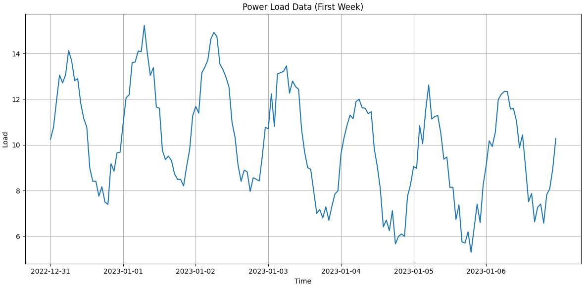
# 可视化原始数据
plt.figure(figsize=(12, 6))
plt.plot(df.index[:168], df['load'].values[:168])  # 显示一周数据
plt.title('Power Load Data (First Week)')
plt.xlabel('Time')
plt.ylabel('Load')
plt.grid(True)
plt.tight_layout()
plt.savefig(os.path.join(result_dir, 'raw_data.png'))
plt.close()

# 数据标准化
scaler = MinMaxScaler(feature_range=(0, 1))
scaled_data = scaler.fit_transform(df['load'].values.reshape(-1, 1)).flatten()

# 创建序列数据
def create_sequences(data, seq_length, pred_length):
    """
    将时间序列转换为输入序列和目标序列
    seq_length: 输入序列长度
    pred_length: 预测序列长度
    """
    X, y = [], []
    for i in range(len(data) - seq_length - pred_length + 1):
        X.append(data[i:i+seq_length])
        y.append(data[i+seq_length:i+seq_length+pred_length])
    return np.array(X), np.array(y)

# 序列长度设置
seq_length = 24 * 7  # 7天数据作为输入
pred_length = 24     # 预测未来24小时

# 创建序列
X, y = create_sequences(scaled_data, seq_length, pred_length)

# 划分训练集、验证集和测试集
X_train_val, X_test, y_train_val, y_test = train_test_split(
    X, y, test_size=0.2, shuffle=False
)
X_train, X_val, y_train, y_val = train_test_split(
    X_train_val, y_train_val, test_size=0.25, shuffle=False  # 0.25 * 0.8 = 0.2
)

# 转换为PyTorch张量
X_train = torch.FloatTensor(X_train).unsqueeze(2)  # 增加特征维度
y_train = torch.FloatTensor(y_train)
X_val = torch.FloatTensor(X_val).unsqueeze(2)
y_val = torch.FloatTensor(y_val)
X_test = torch.FloatTensor(X_test).unsqueeze(2)
y_test = torch.FloatTensor(y_test)

print(f"训练集: X={X_train.shape}, y={y_train.shape}")
print(f"验证集: X={X_val.shape}, y={y_val.shape}")
print(f"测试集: X={X_test.shape}, y={y_test.shape}")

# 创建数据加载器
class TimeSeriesDataset(Dataset):
    def __init__(self, X, y):
        self.X = X
        self.y = y
        
    def __len__(self):
        return len(self.X)
    
    def __getitem__(self, idx):
        return self.X[idx], self.y[idx]

batch_size = 32
train_dataset = TimeSeriesDataset(X_train, y_train)
val_dataset = TimeSeriesDataset(X_val, y_val)
test_dataset = TimeSeriesDataset(X_test, y_test)

train_loader = DataLoader(train_dataset, batch_size=batch_size, shuffle=True)
val_loader = DataLoader(val_dataset, batch_size=batch_size, shuffle=False)
test_loader = DataLoader(test_dataset, batch_size=batch_size, shuffle=False)

Power Load Data

5.3 模型实现

class PositionalEncoding(nn.Module):
    """位置编码模块"""
    def __init__(self, d_model, max_len=5000):
        super(PositionalEncoding, self).__init__()
        
        pe = torch.zeros(max_len, d_model)
        position = torch.arange(0, max_len, dtype=torch.float).unsqueeze(1)
        div_term = torch.exp(torch.arange(0, d_model, 2).float() * (-np.log(10000.0) / d_model))
        
        pe[:, 0::2] = torch.sin(position * div_term)
        pe[:, 1::2] = torch.cos(position * div_term)
        
        pe = pe.unsqueeze(0).transpose(0, 1)
        self.register_buffer('pe', pe)
        
    def forward(self, x):
        # x: (seq_len, batch_size, d_model)
        x = x + self.pe[:x.size(0), :]
        return x

class TransformerLSTM(nn.Module):
    """融合Transformer和LSTM的模型"""
    def __init__(self, input_dim, hidden_dim, transformer_dim, num_heads, num_layers, output_dim):
        super(TransformerLSTM, self).__init__()
        
        # LSTM部分
        self.lstm = nn.LSTM(
            input_size=input_dim,
            hidden_size=hidden_dim,
            num_layers=num_layers,
            batch_first=True,
            dropout=0.2
        )
        
        # Transformer部分
        self.transformer_input_proj = nn.Linear(hidden_dim, transformer_dim)
        self.pos_encoder = PositionalEncoding(transformer_dim)
        transformer_layer = nn.TransformerEncoderLayer(
            d_model=transformer_dim,
            nhead=num_heads,
            dim_feedforward=4*transformer_dim,
            dropout=0.2,
            batch_first=True
        )
        self.transformer_encoder = nn.TransformerEncoder(transformer_layer, num_layers=num_layers)
        
        # 融合层
        self.fusion = nn.Linear(hidden_dim + transformer_dim, hidden_dim)
        
        # 输出层
        self.fc = nn.Sequential(
            nn.Linear(hidden_dim, hidden_dim//2),
            nn.ReLU(),
            nn.Linear(hidden_dim//2, output_dim)
        )
        
        # 融合权重
        self.alpha = nn.Parameter(torch.tensor(0.5))  # 初始化为0.5

    def forward(self, x):
        # x: (batch_size, seq_len, input_dim)
        
        # LSTM特征提取
        lstm_out, _ = self.lstm(x)  # (batch_size, seq_len, hidden_dim)
        lstm_last = lstm_out[:, -1, :]  # 取最后一个时间步的输出
        
        # Transformer特征提取
        transformer_in = self.transformer_input_proj(lstm_out)  # 投影到transformer维度
        transformer_in = self.pos_encoder(transformer_in.transpose(0, 1)).transpose(0, 1)  # 添加位置编码
        transformer_out = self.transformer_encoder(transformer_in)  # (batch_size, seq_len, transformer_dim)
        transformer_last = transformer_out[:, -1, :]  # 取最后一个时间步的输出
        
        # 融合特征
        alpha = torch.sigmoid(self.alpha)  # 确保在[0,1]范围内
        fused = torch.cat([alpha * lstm_last, (1-alpha) * transformer_last], dim=1)
        fused = self.fusion(fused)
        
        # 输出预测
        output = self.fc(fused)
        
        return output

# 模型参数
input_dim = 1  # 输入特征维度
hidden_dim = 64  # LSTM隐藏层维度
transformer_dim = 64  # Transformer维度
num_heads = 4  # 注意力头数
num_layers = 2  # 层数
output_dim = pred_length  # 输出维度（预测长度）

# 初始化模型
model = TransformerLSTM(
    input_dim=input_dim,
    hidden_dim=hidden_dim,
    transformer_dim=transformer_dim,
    num_heads=num_heads,
    num_layers=num_layers,
    output_dim=output_dim
)

# 定义损失函数和优化器
criterion = nn.MSELoss()
optimizer = optim.Adam(model.parameters(), lr=0.001)
scheduler = optim.lr_scheduler.ReduceLROnPlateau(optimizer, 'min', patience=5, factor=0.5)

5.4 模型训练与评估

# 训练模型
device = torch.device('cuda' if torch.cuda.is_available() else 'cpu')
print(f"使用设备: {device}")
model.to(device)

# 训练参数
epochs = 100
patience = 15  # 早停耐心值
best_val_loss = float('inf')
early_stop_counter = 0

# 记录损失
train_losses = []
val_losses = []

start_time = time.time()

for epoch in range(epochs):
    model.train()
    train_loss = 0.0
    
    for batch_X, batch_y in train_loader:
        batch_X, batch_y = batch_X.to(device), batch_y.to(device)
        
        # 前向传播
        outputs = model(batch_X)
        loss = criterion(outputs, batch_y)
        
        # 反向传播和优化
        optimizer.zero_grad()
        loss.backward()
        optimizer.step()
        
        train_loss += loss.item() * batch_X.size(0)
    
    # 计算平均训练损失
    train_loss /= len(train_loader.dataset)
    train_losses.append(train_loss)
    
    # 验证
    model.eval()
    val_loss = 0.0
    
    with torch.no_grad():
        for batch_X, batch_y in val_loader:
            batch_X, batch_y = batch_X.to(device), batch_y.to(device)
            outputs = model(batch_X)
            loss = criterion(outputs, batch_y)
            val_loss += loss.item() * batch_X.size(0)
    
    # 计算平均验证损失
    val_loss /= len(val_loader.dataset)
    val_losses.append(val_loss)
    
    # 学习率调整
    scheduler.step(val_loss)
    
    # 打印 epoch 信息
    print(f'Epoch {epoch+1}/{epochs}, Train Loss: {train_loss:.6f}, Val Loss: {val_loss:.6f}')
    
    # 早停检查
    if val_loss < best_val_loss:
        best_val_loss = val_loss
        torch.save(model.state_dict(), os.path.join(result_dir, 'best_model.pth'))
        early_stop_counter = 0
    else:
        early_stop_counter += 1
        if early_stop_counter >= patience:
            print(f"早停在第 {epoch+1} 轮")
            break

end_time = time.time()
print(f"训练时间: {end_time - start_time:.2f} 秒")

# 绘制训练和验证损失曲线
plt.figure(figsize=(10, 6))
plt.plot(train_losses, label='Training Loss')
plt.plot(val_losses, label='Validation Loss')
plt.title('Training and Validation Loss')
plt.xlabel('Epoch')
plt.ylabel('MSE Loss')
plt.legend()
plt.grid(True)
plt.tight_layout()
plt.savefig(os.path.join(result_dir, 'loss_curve.png'))
plt.close()

# 加载最佳模型
model.load_state_dict(torch.load(os.path.join(result_dir, 'best_model.pth')))
model.to(device)

# 在测试集上评估
model.eval()
test_preds = []
test_actuals = []

with torch.no_grad():
    for batch_X, batch_y in test_loader:
        batch_X = batch_X.to(device)
        outputs = model(batch_X)
        test_preds.extend(outputs.cpu().numpy())
        test_actuals.extend(batch_y.numpy())

# 转换为数组
test_preds = np.array(test_preds)
test_actuals = np.array(test_actuals)

# 反标准化
test_preds_original = scaler.inverse_transform(test_preds.reshape(-1, 1)).reshape(test_preds.shape)
test_actuals_original = scaler.inverse_transform(test_actuals.reshape(-1, 1)).reshape(test_actuals.shape)

# 计算评估指标
mse = mean_squared_error(
    test_actuals_original.flatten(), 
    test_preds_original.flatten()
)
rmse = np.sqrt(mse)
mae = mean_absolute_error(
    test_actuals_original.flatten(), 
    test_preds_original.flatten()
)

print(f"测试集性能:")
print(f"MSE: {mse:.4f}")
print(f"RMSE: {rmse:.4f}")
print(f"MAE: {mae:.4f}")

# 保存评估指标
with open(os.path.join(result_dir, 'metrics.txt'), 'w') as f:
    f.write(f"MSE: {mse:.4f}\n")
    f.write(f"RMSE: {rmse:.4f}\n")
    f.write(f"MAE: {mae:.4f}\n")

5.5 结果可视化

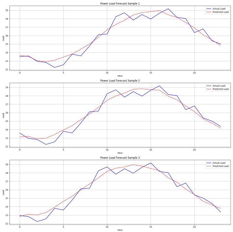
# 可视化预测结果（多个样本）
n_samples = 3
plt.figure(figsize=(15, 5*n_samples))

for i in range(n_samples):
    plt.subplot(n_samples, 1, i+1)
    # 选择第i个测试样本
    actual = test_actuals_original[i]
    pred = test_preds_original[i]
    time_steps = np.arange(len(actual))
    
    plt.plot(time_steps, actual, label='Actual Load', color='blue')
    plt.plot(time_steps, pred, label='Predicted Load', color='red', linestyle='--')
    plt.title(f'Power Load Forecast Sample {i+1}')
    plt.xlabel('Hour')
    plt.ylabel('Load')
    plt.legend()
    plt.grid(True)

plt.tight_layout()
plt.savefig(os.path.join(result_dir, 'forecast_samples.png'))
plt.close()

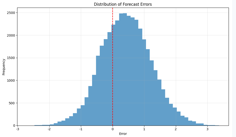
# 可视化预测误差分布
errors = test_actuals_original - test_preds_original
plt.figure(figsize=(10, 6))
plt.hist(errors.flatten(), bins=50, alpha=0.7)
plt.axvline(x=0, color='r', linestyle='--')
plt.title('Distribution of Forecast Errors')
plt.xlabel('Error')
plt.ylabel('Frequency')
plt.grid(True, alpha=0.3)
plt.tight_layout()
plt.savefig(os.path.join(result_dir, 'error_distribution.png'))
plt.close()

# 可视化实际值vs预测值散点图
plt.figure(figsize=(10, 10))
plt.scatter(test_actuals_original.flatten(), test_preds_original.flatten(), alpha=0.5)
# 添加参考线
min_val = min(test_actuals_original.min(), test_preds_original.min())
max_val = max(test_actuals_original.max(), test_preds_original.max())
plt.plot([min_val, max_val], [min_val, max_val], 'r--')
plt.title('Actual vs Predicted Load')
plt.xlabel('Actual Load')
plt.ylabel('Predicted Load')
plt.grid(True, alpha=0.3)
plt.tight_layout()
plt.savefig(os.path.join(result_dir, 'actual_vs_predicted.png'))
plt.close()

# 查看融合权重
print(f"融合权重 alpha: {torch.sigmoid(model.alpha).item():.4f}")
with open(os.path.join(result_dir, 'fusion_weight.txt'), 'w') as f:
    f.write(f"Fusion weight alpha: {torch.sigmoid(model.alpha).item():.4f}\n")

Distribution of Forecast Errors
Power Load Forecast Sample

6. 总结与扩展

本文详细介绍了LSTM和Transformer的原理及其在时间序列预测中的应用，并通过一个电力负荷预测项目展示了如何融合这两种模型。融合模型结合了LSTM处理局部时序依赖的优势和Transformer捕捉全局依赖的能力，在实验中取得了良好的预测效果。

可能的扩展方向：

模型改进：尝试不同的融合策略（如注意力融合、层级融合等）
特征工程：加入外部特征（如温度、节假日等）提高预测精度
超参数优化：使用网格搜索或贝叶斯优化寻找最优参数
多步预测策略：实现递归预测或直接多步预测
不确定性量化：引入概率预测方法，提供预测区间

通过本项目，你可以掌握融合Transformer与LSTM进行时间序列预测的核心方法，并将其应用于其他领域如交通流量预测、股票价格预测等。

DAMO开发者矩阵

DAMO开发者矩阵，由阿里巴巴达摩院和中国互联网协会联合发起，致力于探讨最前沿的技术趋势与应用成果，搭建高质量的交流与分享平台，推动技术创新与产业应用链接，围绕“人工智能与新型计算”构建开放共享的开发者生态。

更多推荐

VLAff：用于统一可操作Affordance的视觉-语言-Affordance模型

DAMO开发者矩阵

学生党写论文别乱堆AI工具：开题、写稿、查重、定稿分别用什么，一篇说清

论文工具别乱堆：从开题到定稿，真正适合学生的 AI 辅助组合很多同学一写论文就问：“ChatGPT、Claude、Kimi、DeepSeek、NotebookLM、毕业之家，到底哪个最强？” 这个问题本身就问错了。大模型负责启发和表达，科研智能体负责文献和流程，查重系统负责风险检测，文献管理工具负责引用规范。它们不是替代关系，而是分工关系。真正高效的用法，是在不同阶段选不同工具，而不是把降重、找