✅作者简介：热爱科研的Matlab仿真开发者，擅长毕业设计辅导、数学建模、数据处理、程序设计科研仿真。

🍎完整代码获取 定制创新 论文复现点击：Matlab科研工作室

 👇 关注我领取海量matlab电子书和数学建模资料 

🍊个人信条：做科研，博学之、审问之、慎思之、明辨之、笃行之，是为：博学慎思，明辨笃行。

🔥 内容介绍

一、引言

同步定位与建图（SLAM）是移动机器人领域的核心问题之一，旨在让机器人在未知环境中实时构建地图并确定自身位置。扩展卡尔曼滤波（EKF）作为一种经典的状态估计方法，在 SLAM 中得到了广泛应用。它能够有效处理机器人运动和传感器测量中的不确定性，通过对机器人状态和地图特征的联合估计，实现精确的定位与建图。

二、SLAM 问题概述

（一）SLAM 的基本概念

SLAM 问题可描述为：机器人在一个未知环境中移动，通过自身携带的传感器（如激光雷达、相机等）获取环境信息。在移动过程中，机器人需要同时估计自身的位姿（位置和姿态）以及构建环境地图。地图可以是基于特征点的地图、栅格地图或拓扑地图等不同形式，而机器人位姿的准确估计是构建精确地图的基础，地图又为机器人的定位提供重要参考，两者相互依赖、相互促进。

（二）SLAM 面临的挑战

1. 不确定性

   ：机器人的运动存在误差，例如车轮打滑、电机控制精度有限等，导致机器人实际运动与预期运动不一致。同时，传感器测量也会引入噪声，如激光雷达测量距离存在误差，相机图像识别可能出现错误。这些不确定性使得准确估计机器人位姿和地图特征变得困难。

2. 计算复杂度

   ：随着机器人在环境中移动，地图中的特征数量不断增加，需要处理的数据量迅速增长。如何在保证估计精度的同时，高效地处理大量数据，是 SLAM 面临的重要挑战之一。

三、扩展卡尔曼滤波（EKF）原理

（一）卡尔曼滤波基础

卡尔曼滤波是一种最优线性递推估计方法，用于处理线性系统中的状态估计问题。它基于系统的状态方程和观测方程，通过预测和更新两个步骤，不断地对系统状态进行估计。在预测步骤中，根据上一时刻的状态估计和系统的动态模型，预测当前时刻的状态；在更新步骤中，利用当前时刻的观测数据对预测状态进行修正，得到更准确的状态估计。

（二）扩展卡尔曼滤波

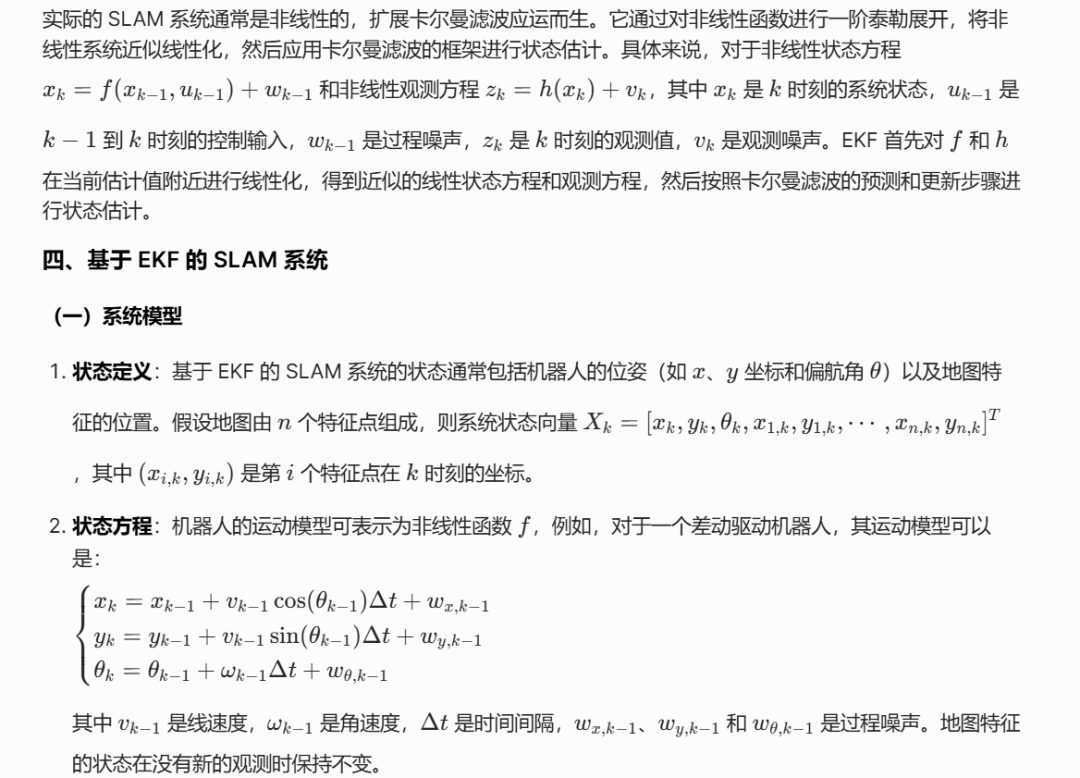
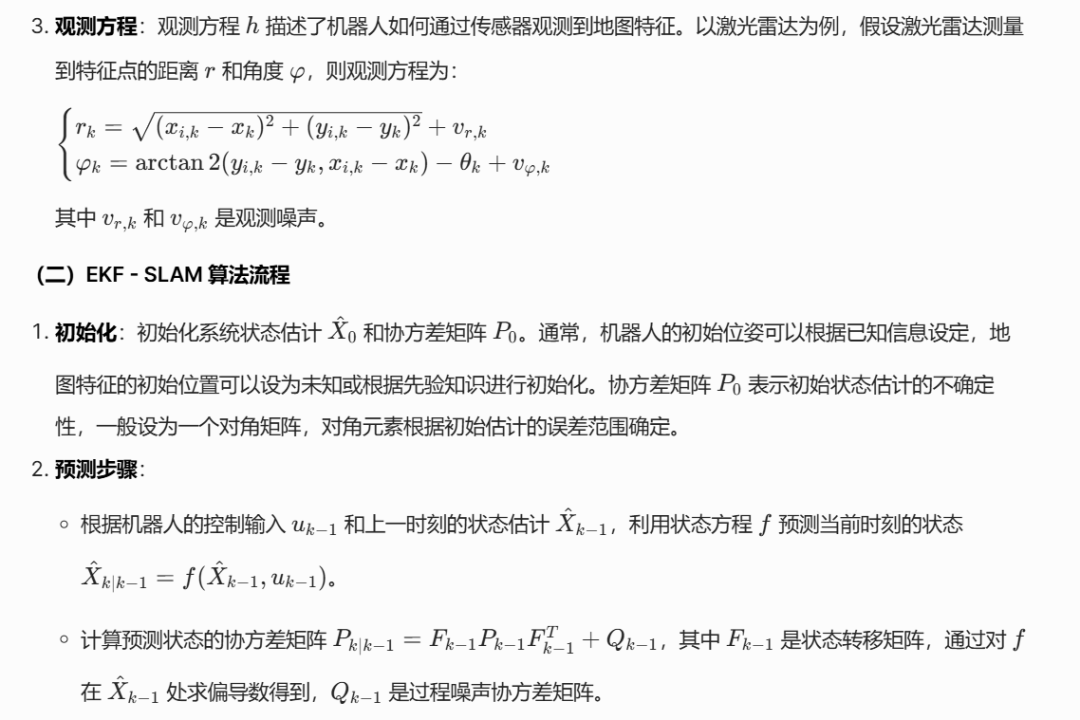
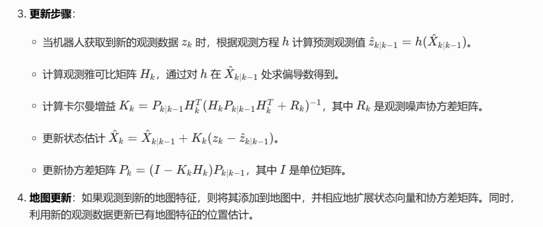
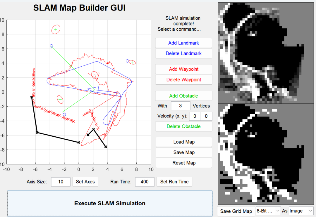
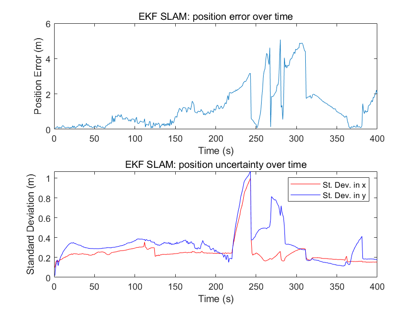
⛳️ 运行结果

📣 部分代码

classdef Robot < handle

    properties

        % Robot properties

        wheelbase       % Width of wheel base (dist. between opposite wheels)

        length          % Length of robot

        R               % True pose [x y a]

        r               % Estimated pose [x y a]

        q               % True system noise

        u               % Control vector [dx da]

        maxspeed        % Maximum speed (m/s)

        min_turn_rad    % Turning radius (m)

        curr_wpt        % Current waypoint reached

    end

    methods

        function rob = Robot                        % Constructor method

            % Default values

            rob.wheelbase =   1;

            rob.length      =   1.5;

            rob.R           =   [0, 0, 0]';

            rob.r           =   rob.R;

            rob.q           =   [0.02;pi/180];       % 2cm, 1 deg

            rob.u           =   [0.1; 0.02];

            rob.maxspeed    =   1.4;                % 1.4m/s ~ 5km/h

            rob.min_turn_rad=   0.5;

            rob.curr_wpt    =   1;

        end

        % Move the robot and obtain new pose and Jacobians.

        %

        % Inputs:

        %   rob             :   Robot object

        %   n               :   Noise (n = [nx na]')

        %   Optional:

        %       strRobType  :   Robot pose to move (true or estimated)

        %

        % Outputs:

        %   r_new           :   New position

        %   RNEW_r          :   Jacobian of r_new wrt. r

        %   RNEW_u          :   Jacobian of r_new wrt. u

        function [r_new, RNEW_r, RNEW_u] = move(rob, n, strRobType)

            if nargin < 3

                % Robot position (p = [x y]') and orientation (a):

                pose = rob.r; a = rob.r(3);

            elseif strcmp(strRobType, 'true')

                pose = rob.R; a = rob.R(3);

            else

                error('strRobType can only take the value "true"');

            end

            % Control input:

            dx = rob.u(1) + n(1);

            da = rob.u(2) + n(2);

            dp = [dx; 0];

            % Determine new orientation

            a_new = a + da;    

            % Ensure that angle is between -pi and pi

            a_new = getPiToPi(a_new);

            if nargout == 1

                % Translate robot to new position in global frame

                p_new = transToGlobal(pose, dp);

            else    % Get Jacobians

                % Translate robot to new position in global frame

                [p_new, PNEW_r, PNEW_dp] = transToGlobal(pose, dp);

                % Jacobians of r_a_new:

                ANEW_a = 1;

                ANEW_da = 1;

                % Hence, Jacobians of r_new:

                RNEW_r = [PNEW_r; 0 0 ANEW_a];

                % We define the perturbation such that it is in the same space

                % as control u. This means that there is uncertainty in how much

                % the robot advances and how much it turns. This means that the

                % Jacobians of RNEW with respect to u are the same as the Jacobian

                % of RNEW with respect to n. Less coding necessary, so a good

                % option.

                RNEW_u = [PNEW_dp(:, 1) zeros(2, 1); 0 ANEW_da];

            end

            r_new = [p_new; a_new];

        end

        % Return the vertices of a triangle of dimensions base*length, 

        % centred at (x, y) and with orientation a.

        %

        % Inputs:

        %   r = [x y a]'        :   local co-ordinate frame of robot

        %   base                :   size of triangle base

        %   length              :   length of triangle

        %

        % Outputs:

        %   p = [x1 x2 x3 x4;

        %        y1 y2 y3 y4] :   vertices of resulting triangle

        function p = computeTriangle(rob, strRobType, r_pos)

            if nargin < 2

                pose = rob.r;

            elseif nargin < 3 && strcmp(strRobType, 'true')

                pose = rob.R;

            elseif nargin < 4

                pose = r_pos;

            else

                error('strRobType can only take the value "True"');

            end

            p = zeros(2, 4);

            p(:, 1) = [-rob.length/3; -rob.wheelbase/2];

            p(:, 2) = [2*rob.length/3; 0];

            p(:, 3) = [-rob.length/3; rob.wheelbase/2;];

            for i = 1:3

                p(:, i) = transToGlobal(pose, p(:, i));

            end

            % We include a fourth point that is equal to the first point in the

            % triangle. This allows us to 'close' the triangle when plotting it

            % using the line function.

            p(:, 4) = p(:, 1);

        end

        function steer(rob, Wpts)

            % Determine if current waypoint reached

            wpt = Wpts(:, rob.curr_wpt);

            % Distance from current waypoint

            dist = sqrt((wpt(1)-rob.R(1))^2 + (wpt(2)-rob.R(2))^2);

            if dist < rob.min_turn_rad

                if rob.curr_wpt < size(Wpts, 2)

                    rob.curr_wpt = rob.curr_wpt + 1;

                else

                    rob.curr_wpt = 1; % Go back to the start

                end

                wpt = Wpts(:, rob.curr_wpt);

            end

            % Change in robot orientation to face current waypoint

            da = getPiToPi(atan2(wpt(2)-rob.R(2), wpt(1)-rob.R(1))-rob.R(3));

            % Amount by which to perturb current robot control:

            dda = da - rob.u(2);

            du = [0; dda];

            rob.setControl(du);

        end

        % Perturb control vector by an amount du = [accel_x; accel_a].

        function u = setControl(rob, du)

            u = rob.u + du;

            % Make sure that angular control is between -pi and pi

            u(2) = getPiToPi(u(2));

            if abs(u(1)) > rob.maxspeed

                % Adjust speed so that max speed isn't exceeded

                u(1) = sign(u(1)) * rob.maxspeed;

            end

            turning_radius = u(1)/u(2);     % Using formula v = omega * r

            if abs(turning_radius) < rob.min_turn_rad

                % Adjust angular velocity so that min turning radius isn't

                % exceeded

            u(2) = sign(u(2)) * abs(u(1)) / rob.min_turn_rad;

            end

            rob.u = u;

        end

    end

end

🔗 参考文献

[1]李永强.基于信息滤波器的同步定位与地图创建技术的研究[D].哈尔滨工业大学[2026-05-10].DOI:CNKI:CDMD:2.2008.195662.

🍅更多免费数学建模和仿真教程关注领取