【优化求解】基于矩阵实编码遗传算法 (MRCGA) 求解机组组合 (UC) 问题附Matlab代码
✅作者简介:热爱科研的Matlab仿真开发者,擅长毕业设计辅导、数学建模、数据处理、建模仿真、程序设计、完整代码获取、论文复现及科研仿真。
🍎 往期回顾关注个人主页:Matlab科研工作室
👇 关注我领取海量matlab电子书和数学建模资料
🍊个人信条:格物致知,完整Matlab代码获取及仿真咨询内容私信。

🔥 内容介绍
一、机组组合 (UC) 问题概述
- 问题定义
:机组组合问题是电力系统调度中的核心任务之一,旨在确定一组发电机组在特定时间段内的开停机状态以及发电功率分配,以满足电力负荷需求,并同时考虑多种约束条件,实现电力系统运行成本最小化、发电效率最大化等目标。例如,在一天 24 小时内,需要合理安排不同类型、不同发电能力的发电机组何时开机、何时关机以及各时段的发电功率,确保既能满足每小时变化的电力负荷,又能保证系统的安全稳定运行,同时尽可能降低发电成本。
- 复杂性与挑战
:UC 问题具有高度的复杂性,这源于其包含众多的约束条件。一方面,有电力平衡约束,即每个时段内所有发电机组的发电功率总和必须等于该时段的电力负荷需求,以保证电力供需平衡。另一方面,发电机组本身存在多种约束,如机组的最小开机时间和最小停机时间限制,这意味着机组一旦开机,必须持续运行一定时间,关机后也需间隔一定时间才能再次开机;还有机组的发电功率上下限约束,规定了机组在运行时的功率输出范围。此外,电力传输网络的约束,如线路传输容量限制,也增加了问题的复杂性。传统的求解方法在处理如此复杂的约束和大规模的决策变量时往往面临计算效率低下和难以找到全局最优解的困境。
二、矩阵实编码遗传算法 (MRCGA) 原理
- 遗传算法基础
:遗传算法是一种模拟生物进化过程的随机搜索优化算法,它借鉴了自然选择和遗传机制。其核心思想是将问题的解编码为个体,这些个体组成种群,通过模拟生物进化中的选择、交叉和变异操作,使种群中的个体不断进化,逐渐接近最优解。
- 矩阵实编码
:在传统遗传算法中,通常采用二进制编码,但对于 UC 问题,二进制编码可能导致编码长度过长,计算效率低下。MRCGA 采用矩阵实编码方式,将机组组合问题的决策变量直接以实数矩阵的形式进行编码。例如,对于一个包含 n 台机组、T 个时段的 UC 问题,可以构建一个 n×T 的矩阵,矩阵中的元素 xit 表示第 i 台机组在第 t 时段的状态(如开机为 1,关机为 0)或发电功率等相关决策变量。这种编码方式更直观地反映了问题的本质,减少了编码和解码的复杂性,提高了算法的计算效率。
- 遗传操作
:
- 选择
:依据个体的适应度值,采用轮盘赌选择、锦标赛选择等策略,从种群中选择出较优的个体,使它们有更大的机会遗传到下一代。适应度函数通常根据 UC 问题的目标函数来设计,如发电成本最小化,适应度值越高表示该个体对应的机组组合方案越优。
- 交叉
:对选择出的个体进行交叉操作,模拟生物遗传中的基因交换过程。在 MRCGA 中,针对矩阵编码的特点,可以采用多种交叉方式,如按行交叉、按列交叉或块交叉等。例如,按行交叉时,随机选择若干行,将两个父代矩阵对应行的元素进行交换,生成新的子代矩阵。交叉操作有助于产生新的解,探索搜索空间。
- 变异
:以一定概率对个体的某些基因进行变异,即对矩阵中的某些元素进行随机改变。例如,将表示机组状态的元素从 1 变为 0 或反之,或者在发电功率限制范围内随机调整发电功率值。变异操作增加了种群的多样性,防止算法过早收敛到局部最优解。
- 选择
三、MRCGA 求解 UC 问题的优势
- 处理复杂约束能力
:MRCGA 在进化过程中,通过适应度函数的设计,可以将 UC 问题的各种复杂约束条件融入其中。例如,对于电力平衡约束,可以在适应度函数中设置惩罚项,当个体对应的机组组合方案不满足电力平衡时,降低其适应度值,引导算法向满足约束的方向进化。对于机组的最小开机和停机时间、发电功率上下限等约束,也可以类似地通过惩罚机制或在遗传操作过程中进行约束处理,确保生成的解在满足所有约束的前提下进行优化。
- 全局搜索能力
:遗传算法的本质特点赋予了 MRCGA 较强的全局搜索能力。通过随机生成初始种群,算法在搜索空间中进行广泛的探索。选择、交叉和变异操作的组合,使得算法能够不断调整搜索方向,跳出局部最优解的陷阱,有更大的机会找到全局最优的机组组合方案。与一些传统的局部搜索算法相比,MRCGA 在处理 UC 问题这样的复杂非凸优化问题时,能够更全面地搜索解空间,提高找到最优解的概率。
- 并行性与可扩展性
:MRCGA 可以很容易地实现并行计算,因为种群中的个体之间相互独立,在进行遗传操作时可以并行处理。这一特性使得算法在处理大规模 UC 问题时,能够利用多核处理器或分布式计算平台,大大提高计算效率。同时,对于不断发展的电力系统,机组数量和时段数量可能不断增加,MRCGA 的可扩展性使其能够适应这种变化,通过适当调整参数和编码方式,继续有效地求解更大规模的 UC 问题。
综上所述,基于矩阵实编码遗传算法 (MRCGA) 为求解机组组合 (UC) 问题提供了一种高效、灵活且具有强大全局搜索能力的方法,能够有效应对 UC 问题的复杂性和大规模性挑战。

⛳️ 运行结果

📣 部分代码
%% MRCGA Unit Commitment - Example Script
% This script demonstrates the use of MRCGA for the 10-unit test system
clear; clc; close all;
%% Define 10-Unit System Data (from paper Appendix B)
units = struct('Pmax', {}, 'Pmin', {}, 'a', {}, 'b', {}, 'c', {}, ...
'Ton', {}, 'Toff', {}, 'HSC', {}, 'CSC', {}, 'CST', {}, ...
'UR', {}, 'DR', {}, 'initial_status', {});
% Unit 1
units(1).Pmax = 455; units(1).Pmin = 150;
units(1).a = 1000; units(1).b = 16.19; units(1).c = 0.00048;
units(1).Ton = 8; units(1).Toff = 8;
units(1).HSC = 4500; units(1).CSC = 9000; units(1).CST = 5;
units(1).UR = 200; units(1).DR = 200;
units(1).initial_status = 8;
% Unit 2
units(2).Pmax = 455; units(2).Pmin = 150;
units(2).a = 970; units(2).b = 17.26; units(2).c = 0.00031;
units(2).Ton = 8; units(2).Toff = 8;
units(2).HSC = 5000; units(2).CSC = 10000; units(2).CST = 5;
units(2).UR = 200; units(2).DR = 200;
units(2).initial_status = 8;
% Unit 3
units(3).Pmax = 130; units(3).Pmin = 20;
units(3).a = 700; units(3).b = 16.6; units(3).c = 0.002;
units(3).Ton = 5; units(3).Toff = 5;
units(3).HSC = 550; units(3).CSC = 1100; units(3).CST = 4;
units(3).UR = 80; units(3).DR = 80;
units(3).initial_status = -5;
% Unit 4
units(4).Pmax = 130; units(4).Pmin = 20;
units(4).a = 680; units(4).b = 16.5; units(4).c = 0.00211;
units(4).Ton = 5; units(4).Toff = 5;
units(4).HSC = 560; units(4).CSC = 1120; units(4).CST = 4;
units(4).UR = 80; units(4).DR = 80;
units(4).initial_status = -5;
% Unit 5
units(5).Pmax = 162; units(5).Pmin = 25;
units(5).a = 450; units(5).b = 19.7; units(5).c = 0.00398;
units(5).Ton = 6; units(5).Toff = 6;
units(5).HSC = 900; units(5).CSC = 1800; units(5).CST = 4;
units(5).UR = 100; units(5).DR = 100;
units(5).initial_status = -6;
% Unit 6
units(6).Pmax = 80; units(6).Pmin = 20;
units(6).a = 370; units(6).b = 22.26; units(6).c = 0.00712;
units(6).Ton = 3; units(6).Toff = 3;
units(6).HSC = 170; units(6).CSC = 340; units(6).CST = 2;
units(6).UR = 50; units(6).DR = 50;
units(6).initial_status = -3;
% Unit 7
units(7).Pmax = 85; units(7).Pmin = 25;
units(7).a = 480; units(7).b = 27.74; units(7).c = 0.00079;
units(7).Ton = 3; units(7).Toff = 3;
units(7).HSC = 260; units(7).CSC = 520; units(7).CST = 2;
units(7).UR = 50; units(7).DR = 50;
units(7).initial_status = -3;
% Unit 8
units(8).Pmax = 55; units(8).Pmin = 10;
units(8).a = 660; units(8).b = 25.92; units(8).c = 0.00413;
units(8).Ton = 1; units(8).Toff = 1;
units(8).HSC = 30; units(8).CSC = 60; units(8).CST = 0;
units(8).UR = 30; units(8).DR = 30;
units(8).initial_status = -1;
% Unit 9
units(9).Pmax = 55; units(9).Pmin = 10;
units(9).a = 665; units(9).b = 27.27; units(9).c = 0.00222;
units(9).Ton = 1; units(9).Toff = 1;
units(9).HSC = 30; units(9).CSC = 60; units(9).CST = 0;
units(9).UR = 30; units(9).DR = 30;
units(9).initial_status = -1;
% Unit 10
units(10).Pmax = 55; units(10).Pmin = 10;
units(10).a = 670; units(10).b = 27.79; units(10).c = 0.00173;
units(10).Ton = 1; units(10).Toff = 1;
units(10).HSC = 30; units(10).CSC = 60; units(10).CST = 0;
units(10).UR = 30; units(10).DR = 30;
units(10).initial_status = -1;
%% 24-Hour Load Demand (MW)
load_demand = [700, 750, 850, 950, 1000, 1100, 1150, 1200, ...
1300, 1400, 1450, 1500, 1400, 1300, 1200, 1050, ...
1000, 1100, 1200, 1400, 1300, 1100, 900, 800];
%% Algorithm Parameters
params = struct();
params.pop_size = 20;
params.max_gen = 500; % 50 * N as per paper
params.crossover_prob = 0.8;
params.row_mutation_prob = 0.8;
params.window_mutation_prob = 0.04;
params.p_replace = 0.05;
params.lambda = 0.6;
%% Run MRCGA
fprintf('Starting MRCGA for 10-unit system...\n');
fprintf('Population Size: %d\n', params.pop_size);
fprintf('Max Generations: %d\n', params.max_gen);
fprintf('======================================\n\n');
tic;
[best_schedule, best_cost, convergence] = MRCGA_UC(units, load_demand, params);
elapsed_time = toc;
fprintf('\nExecution Time: %.2f seconds\n', elapsed_time);
%% Check Constraints
violations = check_constraints(best_schedule, units, load_demand);
display_violations(violations);
%% Display Results
fprintf('\n=== Best Generation Schedule ===\n');
fprintf('Total Cost: $%.2f\n\n', best_cost);
% Display hourly schedule
fprintf('Hour | Load |');
for i = 1:length(units)
fprintf(' U%d |', i);
end
fprintf(' Total |\n');
fprintf('%s\n', repmat('-', 1, 10 + 8*length(units)));
for t = 1:length(load_demand)
fprintf('%4d | %4d |', t, load_demand(t));
for i = 1:length(units)
if best_schedule(i, t) > 0
fprintf(' %3.0f |', best_schedule(i, t));
else
fprintf(' - |');
end
end
fprintf(' %4.0f |\n', sum(best_schedule(:, t)));
end
%% Plot Results
figure('Position', [100, 100, 1200, 800]);
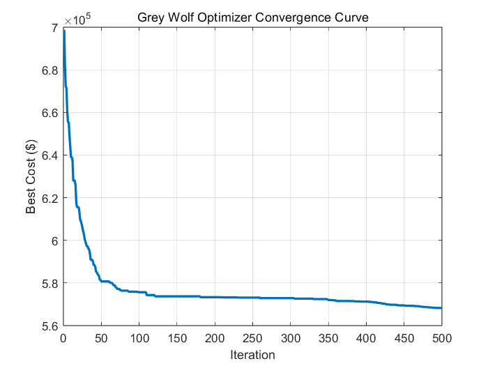
% Subplot 1: Convergence curve
subplot(2, 2, 1);
plot(1:params.max_gen, convergence, 'b-', 'LineWidth', 2);
xlabel('Generation');
ylabel('Best Cost ($)');
title('Convergence Curve');
grid on;
% Subplot 2: Generation Schedule
subplot(2, 2, 2);
hold on;
colors = lines(length(units));
bottom = zeros(1, length(load_demand));
for i = 1:length(units)
bar_data = best_schedule(i, :);
bar(1:24, bar_data, 'stacked');
bottom = bottom + bar_data;
end
plot(1:24, load_demand, 'r-', 'LineWidth', 2);
xlabel('Hour');
ylabel('Power (MW)');
title('Unit Commitment Schedule');
legend([arrayfun(@(x) sprintf('Unit %d', x), 1:length(units), 'UniformOutput', false), {'Load'}]);
grid on;
% Subplot 3: Unit Status
subplot(2, 2, 3);
status_matrix = best_schedule > 0;
imagesc(status_matrix);
colormap([1 1 1; 0 0.5 0]);
xlabel('Hour');
ylabel('Unit');
title('Unit On/Off Status (Green = On, White = Off)');
colorbar('Ticks', [0, 1], 'TickLabels', {'Off', 'On'});
% Subplot 4: Hourly Generation vs Load
subplot(2, 2, 4);
total_gen = sum(best_schedule, 1);
bar(1:24, [load_demand; total_gen]');
xlabel('Hour');
ylabel('Power (MW)');
title('Load vs Total Generation');
legend('Load Demand', 'Total Generation');
grid on;
%% Cost Breakdown
fprintf('\n=== Cost Breakdown ===\n');
total_fuel_cost = 0;
total_startup_cost = 0;
for t = 1:length(load_demand)
for i = 1:length(units)
P = best_schedule(i, t);
if P > 0
fuel_cost = units(i).a + units(i).b * P + units(i).c * P^2;
total_fuel_cost = total_fuel_cost + fuel_cost;
end
% Startup cost calculation
if t == 1
if P > 0 && units(i).initial_status <= 0
off_time = abs(units(i).initial_status);
if off_time > units(i).Toff + units(i).CST
total_startup_cost = total_startup_cost + units(i).CSC;
else
total_startup_cost = total_startup_cost + units(i).HSC;
end
end
else
P_prev = best_schedule(i, t-1);
if P > 0 && P_prev == 0
% Calculate off time
off_time = 0;
for k = t-1:-1:1
if best_schedule(i, k) == 0
off_time = off_time + 1;
else
break;
end
end
if k == 1 && best_schedule(i, 1) == 0 && units(i).initial_status < 0
off_time = off_time + abs(units(i).initial_status);
end
if off_time > units(i).Toff + units(i).CST
total_startup_cost = total_startup_cost + units(i).CSC;
else
total_startup_cost = total_startup_cost + units(i).HSC;
end
end
end
end
end
fprintf('Fuel Cost: $%.2f (%.1f%%)\n', total_fuel_cost, ...
100*total_fuel_cost/best_cost);
fprintf('Startup Cost: $%.2f (%.1f%%)\n', total_startup_cost, ...
100*total_startup_cost/best_cost);
fprintf('Total Cost: $%.2f\n', best_cost);
%% Compare with Literature
fprintf('\n=== Comparison with Literature ===\n');
fprintf('MRCGA Result: $%.2f\n', best_cost);
fprintf('Paper Best: $564,244 (expected)\n');
fprintf('GA1 [24]: $563,977\n');
fprintf('LR [24]: $565,825\n');

🔗 参考文献

🍅往期回顾扫扫下方二维码

DAMO开发者矩阵,由阿里巴巴达摩院和中国互联网协会联合发起,致力于探讨最前沿的技术趋势与应用成果,搭建高质量的交流与分享平台,推动技术创新与产业应用链接,围绕“人工智能与新型计算”构建开放共享的开发者生态。
更多推荐

 0
0 0
0- 0


 已为社区贡献193条内容

所有评论(0)