一、Softmax Loss

$$L=-\sum _{j=1}^T{y}_{j}log(S_j)=-\frac{1}{N}\sum _i\log \left(\frac{e^{{\mathbf{w}}_{y_i}^T{\mathbf{x}}_i}}{{\sum }_j{e}^{{\mathbf{w}}_j^T{\mathbf{x}}_i}}\right)$$

• 首先 $L$ 是损失。
• $S_j$ 是 Softmax的输出向量 $S$ 的第 $j$ 个值，前面已经介绍过了，表示的是这个样本属于第 $j$ 个类别的概率。
• $y_j$ 前面有个求和符号，$j$ 的范围也是 $1$ 到类别数 $T$，因此 $y$ 是一个 $1\times T$ 的向量，里面的 $T$ 个值，而且只有 $1$ 个值是$1$，其他 $T-1$ 个值都是 $0$。那么哪个位置的值是 $1$ 呢？答案是真实标签对应的位置的那个值是 $1$，其他都是 $0$。

1、单个样本 ${\text{x}}^i$ 的 Softmax Loss公式

$$los{s}^i=-\sum _{j=1}^K{y}_{j}log({\hat{y}}_j^i)\stackrel{样本i只属于一个类别j}{=}-log({\hat{y}}_j^i)$$

• 首先 $los{s}^i$ 表示样本 $i$ 的损失。
• ${\hat{y}}_j$ 表示的是样本 $i$ 属于类别 $j$ 的预测概率。
• $y_j$ 表示的是样本 $i$ 属于类别 $j$ 的真实概率；前面有个求和符号，$j$ 的范围也是 $1$ 到类别数 $K$，因此 $y$ 是一个 $1\times K$ 的向量，里面的 $K$ 个值，
  • 多分类任务：如果每个样本只属于一个类别，则只有 $1$ 个值是$1$，其他 $K-1$ 个值都是 $0$。那么哪个位置的值是 $1$ 呢？答案是真实标签对应的位置的那个值是 $1$，其他都是 $0$。
    
    比如：假设类别总数为5类，样本3真实类别为 $c_5$ （多分类任务），则样本3的损失函数：
    $$\begin{array}{rl}los{s}^3=-\sum _{j=1}^K{y}_j^3\cdot log({\hat{y}}_j^3)& =-[y_1^3\cdot log({\hat{y}}_1^3)+y_2^3\cdot log({\hat{y}}_2^3)+y_3^3\cdot log({\hat{y}}_3^3)+y_4^3\cdot log({\hat{y}}_4^3)+y_5^3\cdot log({\hat{y}}_5^3)]\\ & =-[0\cdot log({\hat{y}}_1^3)+0\cdot log({\hat{y}}_2^3)+0\cdot log({\hat{y}}_3^3)+0\cdot log({\hat{y}}_4^3)+1\cdot log({\hat{y}}_5^3)]\\ & =-[1\cdot log({\hat{y}}_5^3)]\\ & =-log({\hat{y}}_5^3)\end{array}$$
  • 多标签分类任务：如果每个样本可以属于多个类别（多标签分类），则可以由 $t$ 个值为 $1$，其他 $K-t$ 个值为 $0$。
    
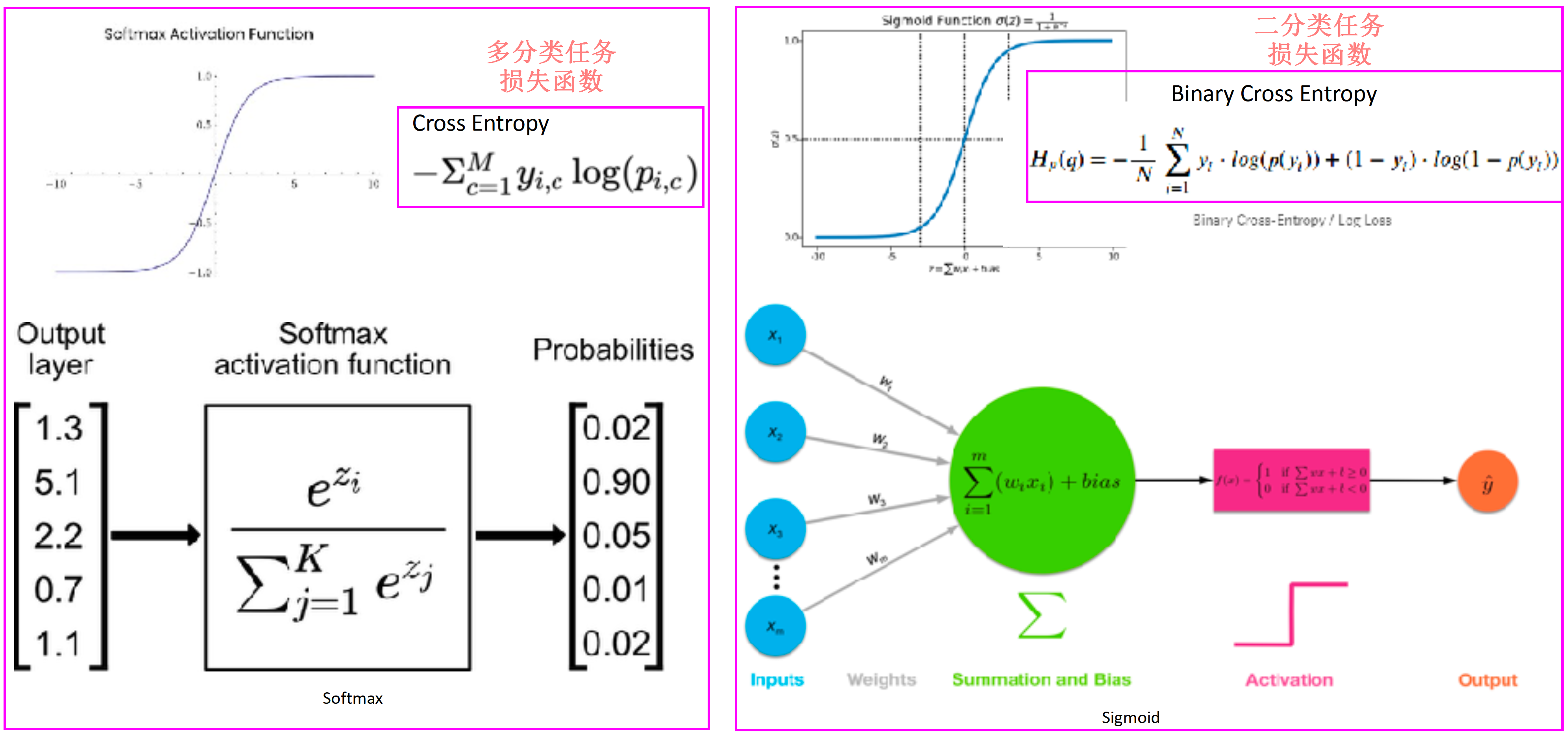
    比如：假设类别总数为5类，样本3真实类别为 $c_1$，$c_5$ （多标签分类任务），则样本3的损失函数：
    $$\begin{array}{rl}los{s}^3=-\sum _{j=1}^K{y}_j^3\cdot log({\hat{y}}_j^3)& =-[y_1^3\cdot log({\hat{y}}_1^3)+y_2^3\cdot log({\hat{y}}_2^3)+y_3^3\cdot log({\hat{y}}_3^3)+y_4^3\cdot log({\hat{y}}_4^3)+y_5^3\cdot log({\hat{y}}_5^3)]\\ & =-[1\cdot log({\hat{y}}_1^3)+0\cdot log({\hat{y}}_2^3)+0\cdot log({\hat{y}}_3^3)+0\cdot log({\hat{y}}_4^3)+1\cdot log({\hat{y}}_5^3)]\\ & =-[1\cdot log({\hat{y}}_1^3)+1\cdot log({\hat{y}}_5^3)]\\ & =-[log({\hat{y}}_1^3)+log({\hat{y}}_5^3)]\end{array}$$

2、样本集 $\text{x}$ 的 Softmax Loss公式（多分类任务，非多标签任务）

$$\begin{array}{rl}Loss& =-\frac{1}{N}\sum _{i=1}^{N}los{s}^i\\ & =-\frac{1}{N}\sum _{i=1}^N\sum _{k=1}^K{y}_k^i\cdot log({\hat{y}}_k^i)\\ & \stackrel{样本i只属于一个类别k}{=}-\frac{1}{N}\sum _{i=1}^{N}log{\hat{y}}_k^i\\ & =-\frac{1}{N}\sum _{i=1}^{N}log[f(z_k^i)]\\ & =-\frac{1}{N}\sum _{i=1}^{N}log\frac{e^{z_k^i}}{{\sum }_{j=1}^K{e}^{z_j^i}}\\ & =-\frac{1}{N}\sum _{i=1}^{N}log\frac{e^{{\text{w}}_k^T{\text{x}}^i}}{{\sum }_{j=1}^K{e}^{{\text{w}}_j^T{\text{x}}^i}}\\ & \stackrel{样本i的真实类别k记为y_i}{=}-\frac{1}{N}\sum _{i=1}^{N}log\frac{e^{{\text{w}}_{y_i}^T{\text{x}}^i}}{{\sum }_{j=1}^K{e}^{{\text{w}}_j^T{\text{x}}^i}}\end{array}$$

其中：

• $N$：表示样本总数量；
• $K$：表示总的类别数量为 $K$；
• $k$：表示样本 ${\text{x}}^i$ 的真实标签类别，记为 $y_i$；
• ${\hat{y}}_k^i$：表示第 $i$ 号样本 ${\text{x}}^i$ 属于类别 $k$ 的预测概率；所有 $K$ 个 ${\hat{y}}_k^i$ 的总和恒等于 $1$；
• ${\text{x}}^i$：表示样本 $i$；
• ${\text{w}}_k^T$：表示第 $k$ 类的权重向量；${\text{w}}_k^T=\left[\begin{array}{ccccccc}{w}_{k,1}& w_{k,2}& w_{k,3}& \cdots & w_{k,n}& \cdots & w_{k,N}\end{array}\right]$；$N$ 表示样本的数据维度；
• ${\text{w}}_j^T$：表示第 $j$ 类的权重向量，其中 $j=1,2,...,K$；

Center Loss

二、L-Softmax Loss（Large Margin Softmax Loss）

相比较Softmax Loss：

• 增加Margin项：角度分类边界之间的空白角度区域
• 增大Margin来提高分类精度
• 缺陷：无法处理W_i≠W_j的情况

$$L_i=-\log \left(\frac{e^{\Vert {\mathbf{w}}_{y_i}\Vert \Vert {\mathbf{x}}_i\Vert \psi ({\theta }_{y_i})}}{e^{\Vert {\mathbf{w}}_{y_i}\Vert \Vert {\mathbf{x}}_i\Vert \psi ({\theta }_{y_i})}+{\sum }_j{e}^{\Vert {\mathbf{w}}_{j\ne y_i}\Vert \Vert {\mathbf{x}}_i\Vert \cos ({\theta }_j)}}\right)\text{\hspace{1em}(4)}$$

其中
$$\psi (\theta )=\{\begin{array}{l}\cos (m\theta ),0\le \theta \le \frac{\pi }{m}\\ \mathcal{D}(\theta ),\frac{\pi }{m}<\theta \le \pi \end{array}\text{\hspace{1em}(5)}$$

• 公式(5)要保证 $D(\theta )$ 要单调递减，并且 $D(\frac{\pi }{m})=cos(\pi )$ ,为了保证随着 ${\theta }_{yi}$ 的增大，样本的损失也增大，需要让 $\psi (\theta )$ 在 $[0,\pi ]$ 单调递减，可以这么理解，如果要让损失函数在样本上递减，必须使得分母 $\left|\left|W_{yi}\right|\right|\left|\left|x_i\right|\right|\psi ({\theta }_{yi})$ 递增，因为 $cos({\theta }_{yi})\ge cos(m{\theta }_{yi})>D({\theta }_{yi})$ ，随着 $\psi ({\theta }_{yi})$ 的递增，可以保证 ${\theta }_{yi}$ 越来越小。
• 总的来说，其实有点类似数学里面的不等式放缩，让原始的Softmax一定小于L-softmax损失，如果L-Softmax损失收敛到一个很小值，那么原始的Softmax损失会比原来更小，这样解决了原始的Softmax损失收敛出现瓶颈的问题

但是为了简化上述(5)的函数，可以改造函数 $\psi (\theta )$ 在 $[0,\pi ]$ 这段区间，因为 $cos(\theta )$ 是周期为 $\pi$ 函数，可以这么如下分析：

• 当 $0\le \theta \le \frac{\pi }{m}$ 时， $\psi (\theta )=cos(m\theta )$
• 当 $\frac{\pi }{m}<\theta \le \frac{2\pi }{m}$ , $\psi (\theta )=-cos(m\theta )-2$ 也就是 $cos(m\theta )$ 在区间 $[\frac{\pi }{m},\frac{2\pi }{m}]$ 对称反转，在向下平移2个单位，与 $[0,\frac{\pi }{m}]$ 这段曲线的右端点相接。
• 当 $\frac{2\pi }{m}<\theta \le \frac{3\pi }{m}$ ， $\psi (\theta )=cos(m\theta )-4$ ，自己画图就可以分析出来；

最终得出论文中 $\psi (\theta )$ 的一般形式：

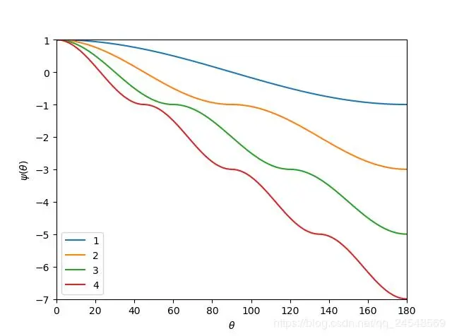
$$\psi (\theta )=(-1{)}^k\cos (m\theta )-2k,\theta \in [\frac{k\pi }{m},\frac{(k+1)\pi }{m}]\text{\hspace{1em}(6)}$$

• 其中 $k+1\le m$ ，所以 $k\in [0,m-1]$ 同时 $k$ 是整数。下图是不同 $m$ 对应的 $\psi (\theta )$曲线
  

在正向传播和反向传播中，我们要计算 $cos({\theta }_{yi})=\frac{W_{yi}{x}_i}{\left|\left|W_{yi}\right|\right|\left|\left|x_i\right|\right|}$ ,然后计算 $cos(m{\theta }_{yi})$，

$\cos (m{\theta }_i)$由下面公式计算

当 $m=1$ 时，L-Softmax Loss就是原来的Softmax Loss。

三、SphereFace（Angular Softmax Loss）

在 L-Softmax Loss 的基础上添加了两个限制条件：

• $||W||=1$
• $b=0$，

使得预测仅取决于 $W$ 和 $x$ 之间的角度。

$$L_{\text{ang}}=\frac{1}{N}\sum _i-\log (\frac{e^{\Vert x_i\Vert \psi ({\theta }_{y_i,i})}}{e^{\Vert x_i\Vert \psi ({\theta }_{y_i,i})}+{\sum }_{j\ne y_i}{e}^{\Vert x_i\Vert \cos ({\theta }_j,i)}})$$

其中：$\psi ({\theta }_{y_i,i})={(-1)}^k\cos (m{\theta }_{y_i,i})-2k$

代码中引入了超参数 $\lambda$，为：

$$\lambda =\max ({\lambda }_{\min },\frac{{\lambda }_{\max }}{1+0.1\times iterator})$$

其中，${\lambda }_{\min }=5$，${\lambda }_{\max }=1500$为程序中预先设定的值。

实际的 $\psi (\theta )$ 为
$$\psi ({\theta }_{y_i})=\frac{{(-1)}^k\cos (m{\theta }_{y_i})-2k+\lambda \cos ({\theta }_{y_i})}{1+\lambda }$$

四、CosFace（Large Margin Cosine Loss）

SphereFace中只对 $W$ 进行归一化。

CosFace的改进：

• 对 $W$ 及 $X$ 均进行了归一化，
• 为了使得训练能收敛，增加了一个参数 $s=30$，

$$\begin{array}{r}{L}_{LMC}=-\frac{1}{N}\sum _{i=1}^N\log \frac{e^{s\cdot [\cos ({\theta }_{y_i},i)-m]}}{e^{s\cdot [\cos ({\theta }_{y_i},i)-m]}+{\sum }_{j=1,j\ne yi}^c{e}^{s\cdot \cos {(\theta }_j,i)}}\end{array}\text{\hspace{1em}(4)}$$

约束条件有：

• $W=\frac{W^{\ast }}{||W^{\ast }||}$
• $x=\frac{x^{\ast }}{||x^{\ast }||}$
• $cos({\theta }_j,i)=W_j^T{x}_i$

其中：

• $N$：训练样本数,
• $x_i$：与$y_i$ 的 ground-truth类对应的第 $i$ 个特征向量；
• $W_j$：$W_j$ 是第 $j$ 类的权重向量；
• ${\theta }_j$： $W_j$ 与 $x_i$的夹角；

五、ArcFace（Additive Angular Margin Loss）

$$\begin{array}{r}{L}_{Arc}=-\frac{1}{N}\sum _{i=1}^{N}log\frac{e^{s[cos({\theta }_{y_i,i}+m)]}}{e^{s[cos({\theta }_{y_i,i}+m)]}+{\sum }_{j\ne y_i}{e}^{scos({\theta }_j,i)}}\end{array}$$

约束条件有：

• $W=\frac{W^{\ast }}{||W^{\ast }||}$
• $x=\frac{x^{\ast }}{||x^{\ast }||}$
• $cos({\theta }_j,i)=W_j^T{x}_i$

其中：

• $N$：训练样本数,
• $x_i$：与$y_i$ 的 ground-truth类对应的第 $i$ 个特征向量；
• $W_j$：$W_j$ 是第 $j$ 类的权重向量；
• ${\theta }_j$： $W_j$ 与 $x_i$的夹角；

可以看到和CosFace非常类似，只是将 $m$ 作为角度加上去了，这样就强行拉大了同类之间的角度，使得神经网络更努力地将同类收得更紧。

There are two main lines of research to train DCNNs for face recognition.

• Those that train a multi-class clas- sifier which can separate different identities in the training set, such by using a softmax classifier [33, 24, 6],
• those that learn directly an embedding, such as the triplet loss[29].

Based on the large-scale training data and the elaborate DCNN architectures, both the softmax-loss-based methods [6] and the triplet-loss-based methods [29] can obtain excellent performance on face recognition.

For the softmax loss:

• (1) the size of the linear transformation matrix W ∈ Rd×n increases linearly with the identities number n; （线性变换矩阵W的大小∈ Rd×n随分类数n线性增加；）
• (2) the learned features are separable for the closed-set classification problem but not discriminative enough for the open-set face recognition problem. （对于闭集分类问题，学习的特征是可分离的，但对于开集人脸识别问题，学习到的特征识别能力不够。）

For the triplet loss:

• (1) there is a combinatorial explosion in the number of face triplets especially for large-scale datasets, leading to a significant increase in the number of iteration steps; （面部三元祖的数量呈组合爆炸式增长，尤其是对于大型数据集，导致迭代步骤的数量显著增加）
• (2) semi-hard sample mining is a quite difficult prob- lem for effective model training.（半硬样本挖掘对于有效的模型训练来说是一个相当困难的问题。）

---

---

---

参考资料：
[6] Q. Cao, L. Shen, W. Xie, O. M. Parkhi, and A. Zisserman. Vggface2: A dataset for recognising faces across pose and age. In FG, 2018. 1, 2, 4, 5, 7, 8
[24] O. M. Parkhi, A. Vedaldi, and A. Zisserman. Deep face recognition. In BMVC, 2015. 1, 2, 6
[29] F. Schroff, D. Kalenichenko, and J. Philbin. Facenet: A unified embedding for face recognition and clustering. In CVPR, 2015. 1, 4, 6, 7
[33] Y. Taigman, M. Yang, M. Ranzato, and L. Wolf. Deepface: Closing the gap to human-level performance in face verifica- tion. In CVPR, 2014. 1, 6
ArcFace