深度学习(7):基于LSTM算法的股票走势预测
·
目标:基于LSTM网络实现对股票走势分析,将股票指数输入LSTM模型训练和推理,最后将判断结果进行输出。
一、原理
先了解RNN,参考博客
好好学习第三天:RNN与股票预测_流萤数点的博客-CSDN博客_rnn 预测
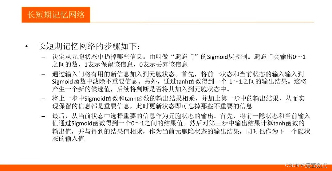
1.了解LSTM算法的基本原理


2.熟悉LSTM趋势预测的常规方法
3.掌握LSTM训练的方法

4.LSTM 和 GRU 是解决短时记忆问题的解决方案,它们具有称为“门”的内部机制,可以调节信息流。


二、过程
1.导入库
import numpy as np
import pandas as pd
import math
import sklearn
import sklearn.preprocessing
import datetime
import os
import matplotlib.pyplot as plt
import tensorflow as tf
2.导入数据
#准备数据,从OSS中获取数据并解压到当前目录:

import oss2
access_key_id = os.getenv('OSS_TEST_ACCESS_KEY_ID', 'LTAI4G1MuHTUeNrKdQEPnbph')
access_key_secret = os.getenv('OSS_TEST_ACCESS_KEY_SECRET', 'm1ILSoVqcPUxFFDqer4tKDxDkoP1ji')
bucket_name = os.getenv('OSS_TEST_BUCKET', 'mldemo')
endpoint = os.getenv('OSS_TEST_ENDPOINT', 'https://oss-cn-shanghai.aliyuncs.com')
# 创建Bucket对象,所有Object相关的接口都可以通过Bucket对象来进行
bucket = oss2.Bucket(oss2.Auth(access_key_id, access_key_secret), endpoint, bucket_name)
# 下载到本地文件
bucket.get_object_to_file('data/c12/stock_data.zip', 'stock_data.zip')![]()
#解压数据
!unzip -o -q stock_data.zip
!rm -rf __MACOSX
!ls stock_data -ilht ![]()
3.可视化
# import all stock prices
df = pd.read_csv("./stock_data/sh300index.csv", index_col = 0)
df.info() 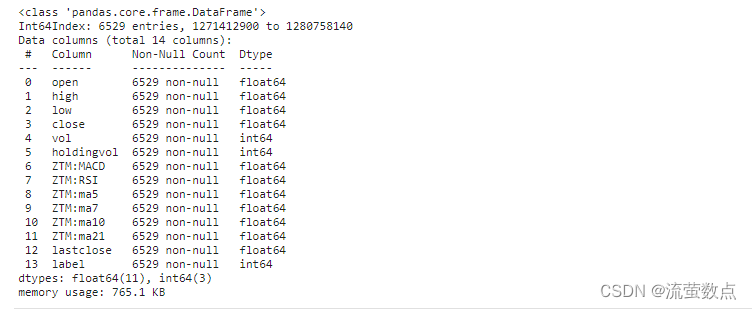
df.head() 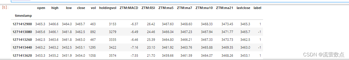
df.describe() 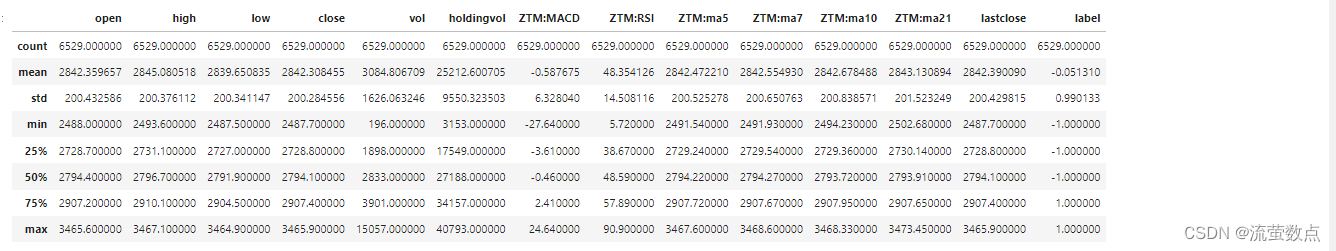
plt.figure(figsize=(15, 5));
plt.subplot(2,1,1);
plt.plot(df.open.values, color='red', label='open')
plt.plot(df.close.values, color='green', label='close')
plt.plot(df.low.values, color='blue', label='low')
plt.plot(df.high.values, color='black', label='high')
plt.title('stock price')
plt.xlabel('time [days]')
plt.ylabel('price')
plt.legend(loc='best')

plt.subplot(2,1,2);
plt.plot(df.vol.values, color='black', label='volume')
plt.title('stock volume')
plt.xlabel('time [days]')
plt.ylabel('volume')
plt.legend(loc='best');
plt.show() 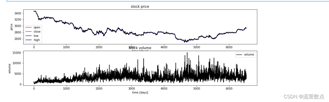
4.数据预处理
# 按照80%/10%/10% 划分训练集、验证集和测试集
valid_set_size_percentage = 10
test_set_size_percentage = 10
# min-max 归一化
def normalize_data(df):
min_max_scaler = sklearn.preprocessing.MinMaxScaler()
df['open'] = min_max_scaler.fit_transform(df.open.values.reshape(-1,1))
df['high'] = min_max_scaler.fit_transform(df.high.values.reshape(-1,1))
df['low'] = min_max_scaler.fit_transform(df.low.values.reshape(-1,1))
df['close'] = min_max_scaler.fit_transform(df['close'].values.reshape(-1,1))
return df# 划分数据集
def load_data(stock, seq_len):
data_raw = stock.to_numpy() # pd to numpy array
data = []
# create all possible sequences of length seq_len
for index in range(len(data_raw) - seq_len):
data.append(data_raw[index: index + seq_len])
data = np.array(data);
valid_set_size = int(np.round(valid_set_size_percentage/100*data.shape[0]));
test_set_size = int(np.round(test_set_size_percentage/100*data.shape[0]));
train_set_size = data.shape[0] - (valid_set_size + test_set_size);
x_train = data[:train_set_size,:-1,:]
y_train = data[:train_set_size,-1,:]
x_valid = data[train_set_size:train_set_size+valid_set_size,:-1,:]
y_valid = data[train_set_size:train_set_size+valid_set_size,-1,:]
x_test = data[train_set_size+valid_set_size:,:-1,:]
y_test = data[train_set_size+valid_set_size:,-1,:]
return [x_train, y_train, x_valid, y_valid, x_test, y_test]# 去除冗余指标
df_stock = df.copy()
df_stock.drop(['vol'],1,inplace=True)
df_stock.drop(['lastclose'],1,inplace=True)
df_stock.drop(['label'],1,inplace=True)
df_stock.drop(['ZTM:ma5'],1,inplace=True)
df_stock.drop(['ZTM:ma7'],1,inplace=True)
df_stock.drop(['ZTM:ma10'],1,inplace=True)
df_stock.drop(['ZTM:ma21'],1,inplace=True)
df_stock.drop(['holdingvol'],1,inplace=True)
df_stock.drop(['ZTM:MACD'],1,inplace=True)
df_stock.drop(['ZTM:RSI'],1,inplace=True)
#查看输入数据
df_stock.head()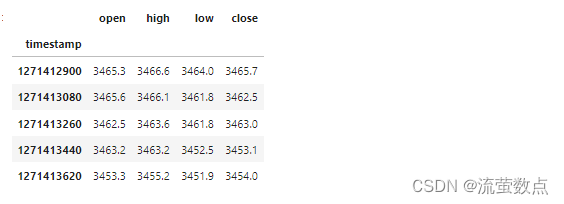
#输出输入列名
cols = list(df_stock.columns.values)
print('df_stock.columns.values = ', cols)![]()
对指标进行归一化处理:
df_stock_norm = normalize_data(df_stock)

# 查看训练集、验证集和测试集情况
seq_len = 20 # 设置最长序列长度
x_train, y_train, x_valid, y_valid, x_test, y_test = load_data(df_stock_norm, seq_len)
print('x_train.shape = ',x_train.shape)
print('y_train.shape = ', y_train.shape)
print('x_valid.shape = ',x_valid.shape)
print('y_valid.shape = ', y_valid.shape)
print('x_test.shape = ', x_test.shape)
print('y_test.shape = ',y_test.shape)
#对指标数据进行可视化
plt.figure(figsize=(15, 6));
plt.plot(df_stock_norm.open.values, color='red', label='open')
plt.plot(df_stock_norm.close.values, color='green', label='close')
plt.plot(df_stock_norm.low.values, color='blue', label='low')
plt.plot(df_stock_norm.high.values, color='black', label='high')
plt.title('stock')
plt.xlabel('time [days]')
plt.ylabel('normalized price/volume')
plt.legend(loc='best')
plt.show()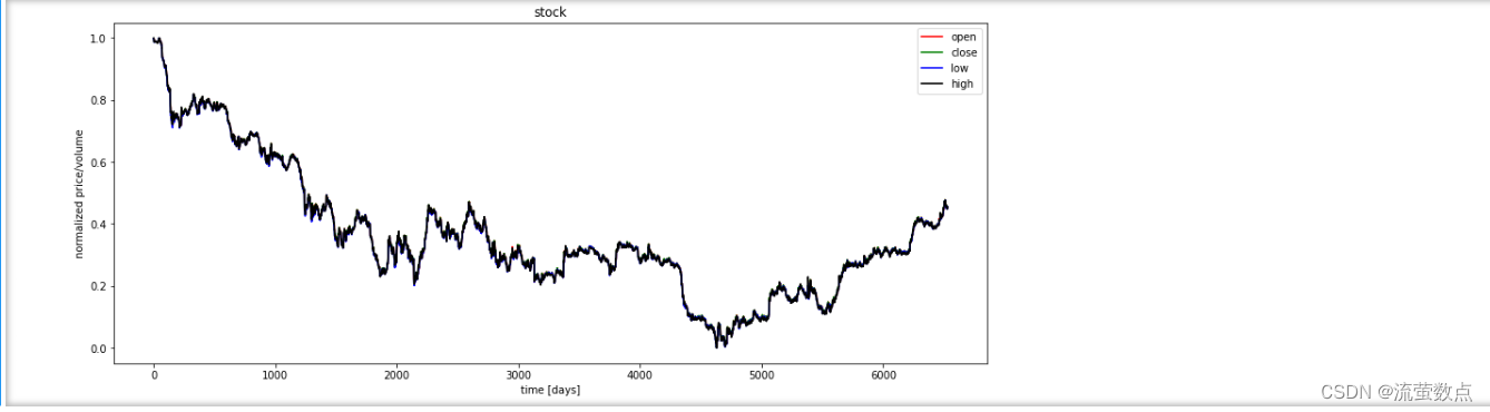
5.RNN建模-LSTM/GRU
#对训练数据随机化处理
index_in_epoch = 0;
perm_array  = np.arange(x_train.shape[0])
np.random.shuffle(perm_array)

# 数据读取方法
def get_next_batch(batch_size):
    global index_in_epoch, x_train, perm_array
    start = index_in_epoch
    index_in_epoch += batch_size

    if index_in_epoch > x_train.shape[0]:
        np.random.shuffle(perm_array) # shuffle permutation array
        start = 0 # start next epoch
        index_in_epoch = batch_size

    end = index_in_epoch
    return x_train[perm_array[start:end]], y_train[perm_array[start:end]]
#定义超参
n_steps = seq_len-1
#输入大小(与指标数量对应)
n_inputs = 4
n_neurons = 200
#输出大小(与指标数量对应)
n_outputs = 4
#层数
n_layers = 2
#学习率
learning_rate = 0.001
#批大小
batch_size = 50
#迭代训练次数
n_epochs = 20
#训练集大小
train_set_size = x_train.shape[0]
#测试集大小
test_set_size = x_test.shape[0]定义网络结构:
tf.reset_default_graph()

X = tf.placeholder(tf.float32, [None, n_steps, n_inputs])
y = tf.placeholder(tf.float32, [None, n_outputs])

# 使用GRU单元结构
layers = [tf.contrib.rnn.GRUCell(num_units=n_neurons, activation=tf.nn.leaky_relu)
         for layer in range(n_layers)]

multi_layer_cell = tf.contrib.rnn.MultiRNNCell(layers)
rnn_outputs, states = tf.nn.dynamic_rnn(multi_layer_cell, X, dtype=tf.float32)

stacked_rnn_outputs = tf.reshape(rnn_outputs, [-1, n_neurons])
stacked_outputs = tf.layers.dense(stacked_rnn_outputs, n_outputs)
outputs = tf.reshape(stacked_outputs, [-1, n_steps, n_outputs])
outputs = outputs[:,n_steps-1,:] # 定义输出

loss = tf.reduce_mean(tf.square(outputs - y)) # 使用MSE作为损失
optimizer = tf.train.AdamOptimizer(learning_rate=learning_rate)
training_op = optimizer.minimize(loss)
开始训练:
# 执行训练
with tf.Session() as sess:
    sess.run(tf.global_variables_initializer())
    for iteration in range(int(n_epochs*train_set_size/batch_size)):
        x_batch, y_batch = get_next_batch(batch_size) # fetch the next training batch
        sess.run(training_op, feed_dict={X: x_batch, y: y_batch})
        if iteration % int(5*train_set_size/batch_size) == 0:
            mse_train = loss.eval(feed_dict={X: x_train, y: y_train})
            mse_valid = loss.eval(feed_dict={X: x_valid, y: y_valid})
            print('%.2f epochs: MSE train/valid = %.6f/%.6f'%(
                iteration*batch_size/train_set_size, mse_train, mse_valid))

    y_train_pred = sess.run(outputs, feed_dict={X: x_train})
    y_valid_pred = sess.run(outputs, feed_dict={X: x_valid})
    y_test_pred = sess.run(outputs, feed_dict={X: x_test})

6.模型应用-预测
对比查看股票指数的历史值和未来值情况:
ft = 0 # 0 = open, 1 = close, 2 = highest, 3 = lowest

#结果可视化
plt.figure(figsize=(15, 5));
plt.subplot(1,2,1);

plt.plot(np.arange(y_train.shape[0]), y_train[:,ft], color='blue', label='train target')

plt.plot(np.arange(y_train.shape[0], y_train.shape[0]+y_valid.shape[0]), y_valid[:,ft],
         color='gray', label='valid target')

plt.plot(np.arange(y_train.shape[0]+y_valid.shape[0],
                   y_train.shape[0]+y_test.shape[0]+y_test.shape[0]),
         y_test[:,ft], color='black', label='test target')

plt.plot(np.arange(y_train_pred.shape[0]),y_train_pred[:,ft], color='red',
         label='train prediction')

plt.plot(np.arange(y_train_pred.shape[0], y_train_pred.shape[0]+y_valid_pred.shape[0]),
         y_valid_pred[:,ft], color='orange', label='valid prediction')

plt.plot(np.arange(y_train_pred.shape[0]+y_valid_pred.shape[0],
                   y_train_pred.shape[0]+y_valid_pred.shape[0]+y_test_pred.shape[0]),
         y_test_pred[:,ft], color='green', label='test prediction')

plt.title('past and future stock prices')
plt.xlabel('time [days]')
plt.ylabel('normalized price')
plt.legend(loc='best');

plt.subplot(1,2,2);

plt.plot(np.arange(y_train.shape[0], y_train.shape[0]+y_test.shape[0]),
         y_test[:,ft], color='black', label='test target')

plt.plot(np.arange(y_train_pred.shape[0], y_train_pred.shape[0]+y_test_pred.shape[0]),
         y_test_pred[:,ft], color='green', label='test prediction')

plt.title('future stock prices')
plt.xlabel('time [days]')
plt.ylabel('normalized price')
plt.legend(loc='best'); 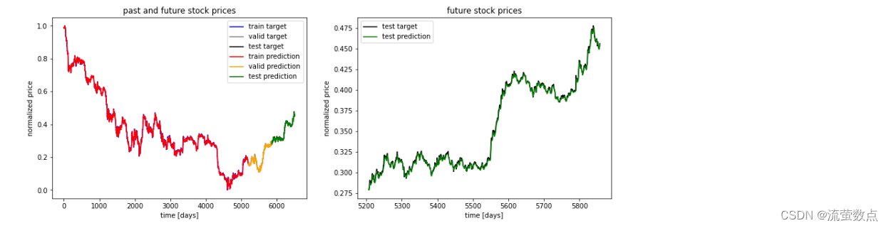

DAMO开发者矩阵,由阿里巴巴达摩院和中国互联网协会联合发起,致力于探讨最前沿的技术趋势与应用成果,搭建高质量的交流与分享平台,推动技术创新与产业应用链接,围绕“人工智能与新型计算”构建开放共享的开发者生态。
更多推荐


 1
1 0
0- 0


 已为社区贡献3条内容

所有评论(0)