10X空间转录组数据分析之细胞niche
作者,Evil Genius
这一篇我们来分享一个关于空间转录组细胞niche的分析方法,我们都知道,通过空间转录组的分析可以形成三个矩阵。
- 分子矩阵 gene X Barcode,就是直接拿到的空间矩阵
- 细胞矩阵 celltype X Barcode(单细胞空间联合分析后的矩阵)
- 生态位表达矩阵 gene(每个位点环境中的表达信息) X Barocde
关于分子矩阵和生态位表达矩阵都是在课程上详细讲过,分析代码也已经分享了,这一篇我们来分享关于细胞矩阵的分析内容,我们的目标是得到下面的分析内容:
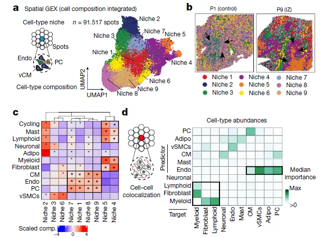
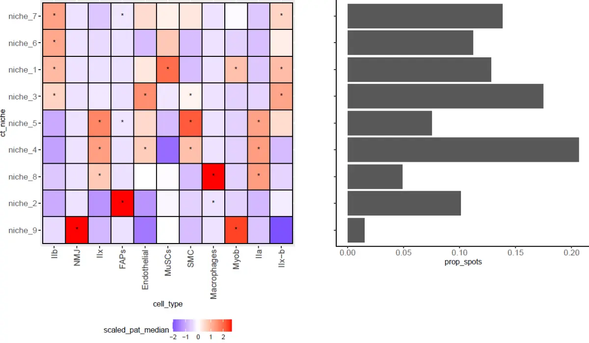
其中a图要实现细胞矩阵的生态位矩阵,b图是niche的空间展示,c图是分析每个niche显著的细胞类型,d图是细胞类型的共定位内容,我们这一篇要实现的是图a,b, c, 图d已经实现过了,通过实例数据实现一下内容(niche的空间分布和细胞类型的显著富集)。
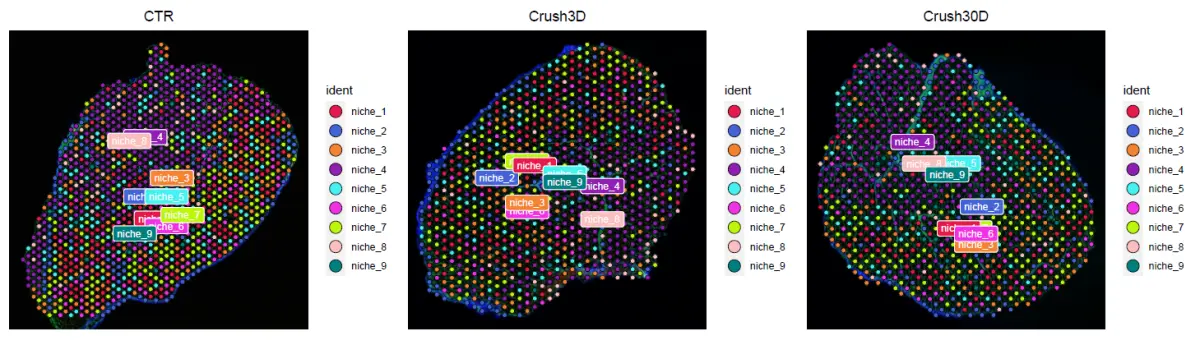
niche空间分布
Niche definitions from spatial transcriptomics data.
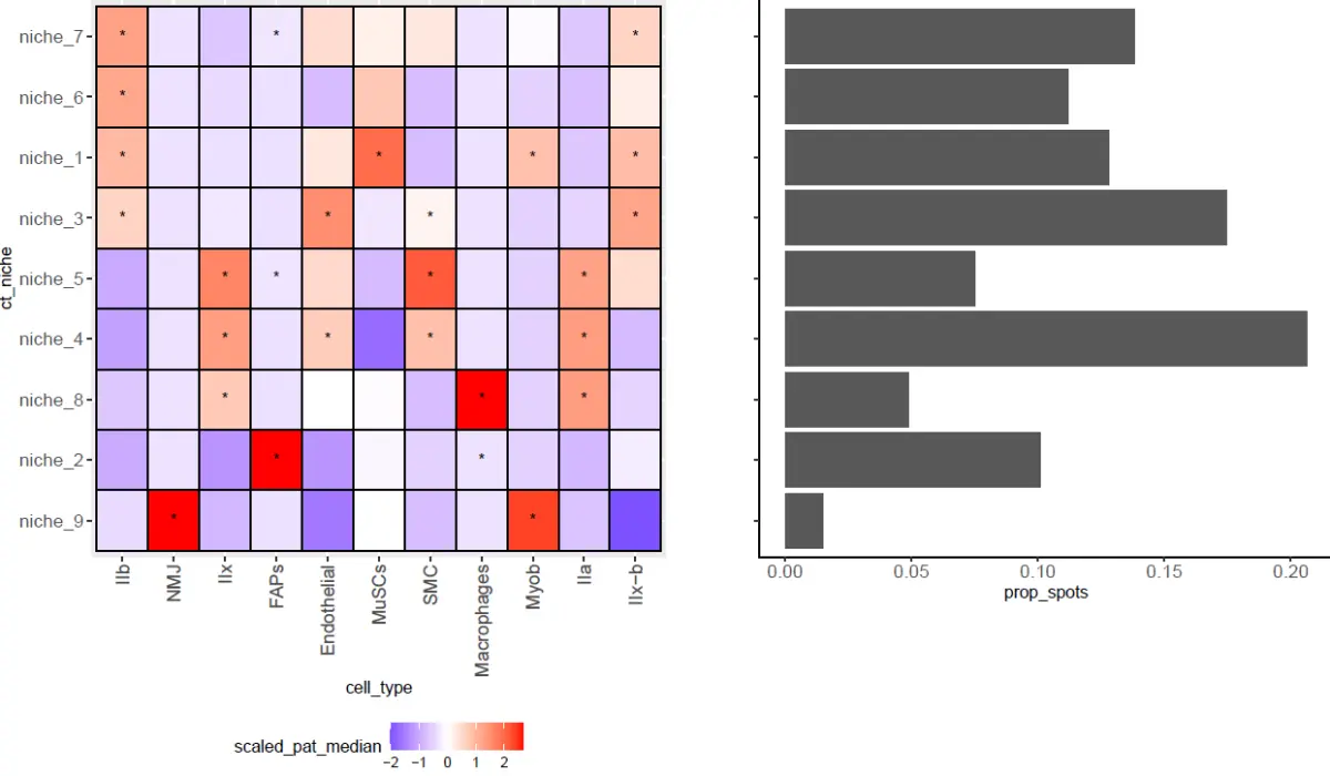
为了确定不同样品中具有相似细胞型组成的斑点组,将每个空间转录组学SPOT和slide的估计细胞型比例转化为等距对数比(ILR),并将SPOT聚类成niche。这些niche代表了细胞组成相似的cluster,代表了不同slide的潜在共享细胞结构;把这些spot群称为细胞niche。使用Wilcoxon检验(FDR < 0.05),通过比较一个细胞类型生态位内细胞类型组成的分布与其他细胞类型的分布,在每个结构中分配了过度代表的细胞类型。通过在每个生态位和其他生态位之间进行Wilcoxon测试来测试给定的细胞状态是否更能代表细胞类型生态位(FDR < 0.05)。
Additionally, to complement the repertoire of niches identified with cell-type compositions, we integrated and clustered the Visium spots of all slides using their log-normalized gene expression. We called these clusters molecular niches. Integration and clustering of spots was performed with the same methodology as the one used to create the snRNA-Seq atlas.
我们来实现一下
加载和读取数据,这里的数据是之前分析的示例数据
suppressMessages({
library(Seurat)
library(compositions)
library(tidyverse)
library(clustree)
library(uwot)
library(scran)
library(cluster)
library(RColorBrewer)
})

adata = readRDS('/root/singlepipeline/demodata/Muscle.spatial.rds')
提取细胞矩阵,这个矩阵就是单细胞空间联合分析的矩阵,默认Seurat的分析结果,其他软件的分析结果可以进行完整替换。
integrated_compositions <- t(adata@assays$predictions@data)

integrated_compositions = integrated_compositions[,-which(colnames(integrated_compositions) %in% c("max"))]
对细胞矩阵进行处理,这里的处理根据矩阵的特性与分子矩阵的处理完全不同,需要大家详细分析一下。
if (max(integrated_compositions) <= 1){integrated_compositions = integrated_compositions * 20}

baseILR <- ilrBase(x = integrated_compositions,method = "basic")

cell_ilr <- as.matrix(ilr(integrated_compositions, baseILR))

colnames(cell_ilr) <- paste0("ILR_", 1:ncol(cell_ilr))

# Make community graph
k_vect <- c(10, 20, 30)

k_vect <- set_names(k_vect, paste0("k_",k_vect))

cluster_info <- map(k_vect, function(k) {

print(k)

print("Generating SNN")

snn_graph <- scran::buildSNNGraph(x = t(cell_ilr %>% as.data.frame() %>% as.matrix()), k = k)

print("Louvain clustering")

clust.louvain <- igraph::cluster_louvain(snn_graph)

clusters <- tibble(cluster = clust.louvain$membership,spot_id = rownames(cell_ilr))

})

cluster_info <- cluster_info %>% enframe() %>% unnest() %>% pivot_wider(names_from = name,values_from = cluster)


# Create UMAP and plot the compositions
comp_umap <- umap(cell_ilr, n_neighbors = 30, n_epochs = 1000,metric = "cosine") %>%  as.data.frame() %>% as.data.frame() %>% mutate(row_id = rownames(cell_ilr))

comp_umap <- comp_umap[, 1:3]

comp_umap <- comp_umap %>% left_join(cluster_info, by = c("row_id" = "spot_id"))


# Make the niche annotation meta-data

cluster_info <- comp_umap %>% dplyr::select(c("row_id","k_30")) %>% dplyr::rename("niche" = k_30) %>% dplyr::mutate(ct_niche = paste0("niche_", niche))

# What are the cells that define the niches?

niche_summary_pat <- integrated_compositions %>% as.data.frame() %>% rownames_to_column("row_id") %>% pivot_longer(-row_id,values_to = "ct_prop", names_to = "cell_type") %>% left_join(cluster_info) %>% mutate(orig.ident = strsplit(row_id, "[..]") %>% map_chr(., ~ .x[1])) %>% group_by(orig.ident, ct_niche, cell_type) %>% summarize(median_ct_prop = median(ct_prop))

niche_summary <- niche_summary_pat %>% ungroup() %>% group_by(ct_niche, cell_type) %>% summarise(patient_median_ct_prop = median(median_ct_prop))

# Data manipulation to have clustered data

niche_summary_mat <- niche_summary %>% pivot_wider(values_from = patient_median_ct_prop, names_from =  cell_type, values_fill = 0) %>%
 column_to_rownames("ct_niche") %>% as.matrix()

niche_order <- hclust(dist(niche_summary_mat))

niche_order <- niche_order$labels[niche_order$order]

ct_order <- hclust(dist(t(niche_summary_mat)))

ct_order <- ct_order$labels[ct_order$order]

# Find characteristic cell types of each niche
# We have per patient the proportion of each cell-type in each niche

run_wilcox_up <- function(prop_data) {

prop_data_group <- prop_data[["ct_niche"]] %>% unique() %>% set_names()

  map(prop_data_group, function(g) {

    test_data <- prop_data %>% mutate(test_group = ifelse(ct_niche == g,"target", "rest")) %>% mutate(test_group = factor(test_group,levels = c("target", "rest")))

    wilcox.test(median_ct_prop ~ test_group, data = test_data, alternative = "greater") %>% broom::tidy()
  }) %>% enframe("ct_niche") %>% unnest()

}

wilcoxon_res <- niche_summary_pat %>%
  ungroup() %>%
  group_by(cell_type) %>%
  nest() %>%
  mutate(wres = map(data, run_wilcox_up)) %>%
  dplyr::select(wres) %>%
  unnest() %>%
  ungroup() %>%
  mutate(p_corr = p.adjust(p.value))

wilcoxon_res <- wilcoxon_res %>% mutate(significant = ifelse(p_corr <= 0.15, "*", ""))

write.table(niche_summary_pat, file = "./niche_summary_pat.txt", col.names = T, row.names = F, quote = F, sep = "\t")

write.table(wilcoxon_res, file = "./wilcoxon_res_cells_niches.txt",col.names = T, row.names = F, quote = F, sep = "\t")

head(niche_summary_pat)
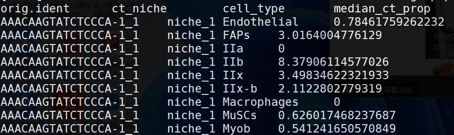
head(wilcoxon_res)

mean_ct_prop_plt <- niche_summary %>%
  left_join(wilcoxon_res, by = c("ct_niche", "cell_type")) %>%
  mutate(cell_type = factor(cell_type, levels = ct_order),
         ct_niche = factor(ct_niche, levels = niche_order)) %>%
  ungroup() %>%
  group_by(cell_type) %>%
  mutate(scaled_pat_median = (patient_median_ct_prop - mean(patient_median_ct_prop))/sd(patient_median_ct_prop)) %>%
  ungroup() %>%
  ggplot(aes(x = cell_type, y = ct_niche, fill = scaled_pat_median)) +
  geom_tile() +
  geom_text(aes(label = significant)) +
  theme(axis.text.x = element_text(angle = 90, hjust = 1, vjust = 0.5, size = 12),
        legend.position = "bottom",
        plot.margin = unit(c(0, 0, 0, 0), "cm"),
        axis.text.y = element_text(size=12)) +
  scale_fill_gradient2(high = "red",mid = 'white', low = "blue")


# Finally describe the proportions of those niches in all the data
cluster_counts <- cluster_info %>%
  dplyr::select_at(c("row_id", "ct_niche")) %>%
  group_by(ct_niche) %>%
  summarise(nspots = length(ct_niche)) %>%
  mutate(prop_spots = nspots/sum(nspots))

write_csv(cluster_counts, file = "./niche_prop_summary.csv")
可视化,主要是每个Niche的细胞类型的富集情况,也是我们分析的重点,也是文献中的重点内容。
barplts <- cluster_counts %>%
  mutate(ct_niche = factor(ct_niche, levels = niche_order)) %>%
  ggplot(aes(y = ct_niche, x = prop_spots)) +
  geom_bar(stat = "identity") +
  theme_classic() + ylab("") +
  theme(axis.text.y = element_blank(),
        plot.margin = unit(c(0, 0, 0, 0), "cm"),
        axis.text.x = element_text(size=12))

niche_summary_plt <- cowplot::plot_grid(mean_ct_prop_plt, barplts, align = "hv", axis = "tb")

pdf('characteristic_ct_niches.pdf',width = 12,height = 7)

plot(niche_summary_plt)

dev.off()
adata = adata[,cluster_info$row_id]

Idents(adata) = cluster_info$ct_niche

sample_cols = unique(c(brewer.pal(8,"Dark2"),brewer.pal(9,"Set1"),brewer.pal(8,"Set2"),brewer.pal(12,"Set3")))
defined_cols = c('#e6194b', '#4363d8', '#f58231', '#911eb4', '#46f0f0', '#f032e6', '#bcf60c', '#fabebe', '#008080', '#e6beff', '#9a6324', '#fffac8', '#800000', '#aaffc3', '#808000', '#ffd8b1', '#000075', '#808080', sample_cols)

p = SpatialDimPlot(adata, label = TRUE, label.size = 3)

for (i in 1:length(p)){p[[i]] = p[[i]] + guides(fill=guide_legend(override.aes = list(size=5))) + scale_fill_manual(values = defined_cols) }

pdf('niche.spatial.pdf',width = 15)

print(p)

dev.off()
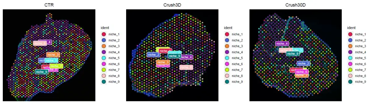
这个需要大家根据自己的数据进行详细的数据分析了,这个分析内容很重要,希望引起大家的重视。
生活很好,有你更好

DAMO开发者矩阵,由阿里巴巴达摩院和中国互联网协会联合发起,致力于探讨最前沿的技术趋势与应用成果,搭建高质量的交流与分享平台,推动技术创新与产业应用链接,围绕“人工智能与新型计算”构建开放共享的开发者生态。
更多推荐



 3
3 0
0- 0


 已为社区贡献57条内容

所有评论(0)