[机器学习]多变量线性回归代码实现
·
[机器学习]多变量线性回归代码实现
dataset
2104,3,399900
1600,3,329900
2400,3,369000
1416,2,232000
3000,4,539900
1985,4,299900
1534,3,314900
1427,3,198999
1380,3,212000
1494,3,242500
1940,4,239999
2000,3,347000
1890,3,329999
4478,5,699900
1268,3,259900
2300,4,449900
1320,2,299900
1236,3,199900
2609,4,499998
3031,4,599000
1767,3,252900
1888,2,255000
1604,3,242900
1962,4,259900
3898,3,573900
1100,3,249900
1458,3,464500
2526,3,469000
2200,3,475000
2637,3,299900
import numpy as np
import pandas as pd
import matplotlib.pyplot as plt
data = pd.read_csv("ex1data2.txt",names = ["size","bedrooms","price"])
print(data.head())
def normalize_feature(data):
return (data - data.mean())/data.std()
data = normalize_feature(data)
print(data.head())
plt.scatter(data["size"],data["price"],label = "size")
plt.scatter(data["bedrooms"],data["price"],label = "bedrooms")
plt.legend()
data.insert(0,"ones",1)
X = data.iloc[:,0:-1]
y = data.iloc[:,-1]
X = X.values
y = y.values
print(X.shape)
y = y.reshape(30,1)
print(y.shape)
def costFunction(X, y, theta):
inner = np.power(X @ theta - y, 2)
return np.sum(inner) / (2 * len(X))
theta = np.zeros((3,1))
cost_init = costFunction(X,y,theta)
print(cost_init)
# 梯度下降
def gradientDescent(X, y, theta, alpha, iters,isprint=False):
costs = []
m = len(X) # 获取样本数量
for i in range(iters):
predictions = X @ theta
errors = predictions - y
gradient = X.T @ errors / m
theta -= alpha * gradient
cost = costFunction(X, y, theta)
costs.append(cost)
if i % 100 == 0:
if isprint:
print(f"Cost after iteration {i}: {cost}")
return theta, costs
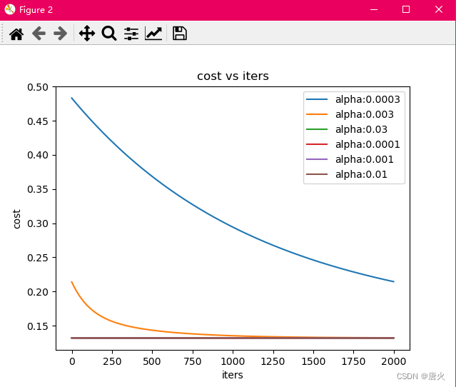
# 不同alpha下的效果
candidate_alpha = [0.0003,0.003,0.03,0.0001,0.001,0.01]
iters = 2000
fig,ax = plt.subplots()
for alpha in candidate_alpha:
_,costs = gradientDescent(X,y,theta,alpha,iters)
ax.plot(np.arange(iters),costs,label = "alpha:{}".format(alpha))
ax.set(xlabel = "iters",ylabel = "cost",title = "cost vs iters")
plt.legend()
plt.show()
运行结果: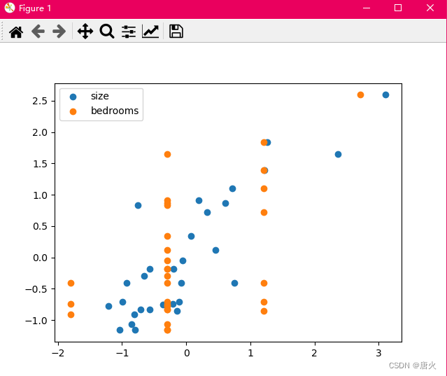

DAMO开发者矩阵,由阿里巴巴达摩院和中国互联网协会联合发起,致力于探讨最前沿的技术趋势与应用成果,搭建高质量的交流与分享平台,推动技术创新与产业应用链接,围绕“人工智能与新型计算”构建开放共享的开发者生态。
更多推荐
 5
5 0
0- 0


 已为社区贡献5条内容

所有评论(0)