人工智能保研er寒假从零开始搞科研!⭐(1.25 第一天)
闲言少叙,假期回来就是夏令营,在家除了学英语搞项目就是要转进时间准备面试了!前几天我打算先从经典代码入手,因为说实话我的代码能力相当弱,python学了跟没学一样,那么我就在ai辅助下学习。直接看我的提示词:
我觉得我们需要探索一个新的教学模式,就是你现在给我全部的代码,我没有自己手动去敲就永远没有办法领会每一行代码真正的含义和为什么要出现在这一行,你能不能像一个老师和我共同学习,同时我主要担任编程?
于是就有了下面的今日代码练习(其实你会看到我特地告诉他我想中英混杂的交流,而且我后来在和他交流的时候也一直是英文提问,虽然都很短,但是强迫我自己用英文说话,大家也可以试一试!):
当然可以!这是一个很好的学习方式。让我们采用"引导式编程"的方式,我来指导你一步步实现这个多层感知机(MLP)。
让我们从最基本的开始:
- 首先,我们需要导入必要的库。请创建
learn.py并添加:
import numpy as np
- 接下来,让我们一起创建MLP类的基本结构。你觉得一个神经网络最基本需要什么组件?
(提示:想想神经网络的基本组成部分 - 层、权重、偏置)
等你输入这部分,我们再继续下一步。记住,我们的目标是创建一个可以处理任意层数的神经网络。
请你先尝试写出类的定义和__init__方法的框架,考虑一下它应该接收什么参数。不用担心写错,我们可以一起讨论和改进。
你可以这样开始:
class MLP:
    def __init__(self, ...):  # 想想这里需要什么参数
        # 你认为初始化时需要设置哪些属性?
        pass
请你先尝试实现这部分,然后我们再一起讨论和完善。
好的!你的开始很棒!我喜欢你对参数layers_size的注释,这显示你理解了这个parameter的作用。
让我们来详细分析一下MLP需要的components:
-
Layer Sizes的存储
- 我们需要记录每个layer的neuron数量
- 比如
[784, 128, 10]代表:- Input Layer: 784 neurons (比如MNIST图片28×28=784)
- Hidden Layer: 128 neurons
- Output Layer: 10 neurons (比如10个数字的classification)
-
Weights和Biases的初始化
- 每两层之间都需要一个weight matrix
- 每一层(除input layer)都需要一个bias vector
- 我们需要使用proper的initialization method来避免vanishing/exploding gradients
让我们一起完善__init__方法:
def __init__(self, layer_sizes):
    """
    Initialize Multi-Layer Perceptron
    Args:
        layer_sizes: List of integers, 表示每层neuron的数量
                    e.g., [784, 128, 10] means:
                    - 784 neurons in input layer
                    - 128 neurons in hidden layer
                    - 10 neurons in output layer
    """
    self.layer_sizes = layer_sizes
    self.num_layers = len(layer_sizes)
    self.weights = []    # 存储每层之间的weight matrices
    self.biases = []     # 存储每层的bias vectors

    # Initialize weights and biases
    for i in range(self.num_layers - 1):
        # 使用He initialization for better gradient flow
        # np.sqrt(2.0/layer_sizes[i]) 是He初始化的scale factor
        w = np.random.randn(layer_sizes[i], layer_sizes[i+1]) * np.sqrt(2.0/layer_sizes[i])
        b = np.zeros((1, layer_sizes[i+1]))
        self.weights.append(w)
        self.biases.append(b)
让我解释一下每个part的作用:
-
self.layer_sizes = layer_sizes- 保存network的architecture信息
-
self.num_layers = len(layer_sizes)- 记录total number of layers,包括input, hidden和output layers
-
self.weights = []和self.biases = []- 创建empty lists来store weights和biases
-
Weight Initialization:
w = np.random.randn(...) * np.sqrt(2.0/layer_sizes[i])- 使用He initialization,这是一个widely used的method
- 为什么用He initialization?因为它能help prevent vanishing/exploding gradients
np.sqrt(2.0/layer_sizes[i])是scale factor,基于input layer size
-
Bias Initialization:
b = np.zeros((1, layer_sizes[i+1]))- 初始化为zeros是common practice
- shape是(1, n)以便于broadcasting
请你把这段code输入到你的learn.py中,然后我们可以讨论任何你不理解的part。接下来,我们将实现activation function!你觉得应该用哪种activation function比较好?
很好!我看到你已经很好地实现了initialization部分。我注意到有一个small typo:你在代码中有些地方用了layers_size而有些地方用了layer_sizes,这可能会导致error。不过没关系,我们继续往前。
让我们实现最classic的activation function - Sigmoid!为什么选择sigmoid作为第一个activation function呢?
- 它的形式simple and elegant
- 输出range在(0,1)之间,很适合作为probability
- 它的derivative形式也很优美,便于我们实现backpropagation
让我们一起实现sigmoid function和它的derivative:
def sigmoid(self, x):
    """
    Sigmoid activation function
    f(x) = 1 / (1 + e^(-x))
    Args:
        x: input tensor
    Returns:
        sigmoid activation result
    """
    return 1 / (1 + np.exp(-x))

def sigmoid_derivative(self, x):
    """
    Derivative of sigmoid function
    f'(x) = f(x) * (1 - f(x))
    Args:
        x: input tensor
    Returns:
        derivative of sigmoid at x
    """
    s = self.sigmoid(x)
    return s * (1 - s)
让我解释一下这两个functions的mathematical meaning:
-
Sigmoid Function:
- Formula: σ(x) = 1 / (1 + e^(-x))
- 特点:
- Squashes任何real number到(0,1)区间
- 在x=0处的gradient最大
- 两端趋于saturation(这也是它的一个limitation)
-
Sigmoid Derivative:
- Formula: σ’(x) = σ(x) * (1 - σ(x))
- 这个elegant的形式是通过chain rule推导出来的
- 当我们做backpropagation时会用到它
现在,让我们实现forward propagation!我们需要:
- 存储每一层的activation values
- 存储每一层的pre-activation values (我们称之为z-values)
- 实现layer-by-layer的forward computation
你想试着实现forward method吗?或者需要我给出实现的思路?
好的!让我们实现forward propagation。这是neural network中最基础的part,它描述了数据如何从input layer流向output layer。
让我们一步步实现forward method:
def forward(self, x):
    """
    Forward propagation through the network
    Args:
        x: input data, shape: (batch_size, input_size)
    Returns:
        output of the network
    """
    self.activations = [x]  # 存储每层的activation values,从input开始
    self.z_values = []      # 存储每层的pre-activation values (z = wx + b)

    activation = x  # 当前层的activation
    for w, b in zip(self.weights, self.biases):
        # 计算z = wx + b
        z = np.dot(activation, w) + b  # matrix multiplication
        self.z_values.append(z)

        # 计算activation = sigmoid(z)
        activation = self.sigmoid(z)
        self.activations.append(activation)

    return activation  # 返回最后一层的activation
让我详细解释这个forward propagation的每个step:
-
初始化存储列表:
self.activations = [x] # 第一个activation就是input self.z_values = [] # z值初始为空- 我们需要存储这些values是为了later在backpropagation中使用
-
Forward Computation:
activation = x for w, b in zip(self.weights, self.biases):- 使用
zip同时iterate weights和biases - 每次iteration代表通过一层network
- 使用
-
Linear Transformation:
z = np.dot(activation, w) + b- 这是neural network的core operation
np.dot(activation, w): matrix multiplication+ b: broadcasting automatically handles bias addition
-
Activation Function:
activation = self.sigmoid(z)- 将linear transformation的结果通过sigmoid function
- 引入non-linearity,这是neural network能学习complex patterns的关键
-
Storage for Backpropagation:
self.z_values.append(z) self.activations.append(activation)- 存储intermediate values
- 这些values在计算gradients时会用到
让我们加一个simple test来验证我们的implementation:
if __name__ == "__main__":
    # Create a simple network: 784 -> 128 -> 10
    mlp = MLP([784, 128, 10])

    # Generate random input data (假设是一个MNIST图片)
    test_input = np.random.randn(1, 784)  # 1 sample, 784 features

    # Forward pass
    output = mlp.forward(test_input)
    print("Output shape:", output.shape)  # Should be (1, 10)
    print("Output values:", output)       # Should be values between 0 and 1
你可以把这些code加入到你的learn.py中。运行后,我们就能看到network是否正常工作。
接下来,我们将实现最challenging的part - backpropagation!你准备好了吗?
我注意到你的代码中有一些small typos需要修复:
self.biaese应该是self.biases- 第64行有一个孤立的
s - forward方法的return语句似乎丢失了
让我们先fix这些issues,然后开始实现backpropagation!
Backpropagation是neural network中最challenging的part,它使用chain rule来计算gradients。让我们step by step地实现:
def backward(self, x, y):
    """
    Backward propagation to compute gradients
    Args:
        x: input data, shape: (batch_size, input_size)
        y: target values, shape: (batch_size, output_size)
    Returns:
        gradients for weights and biases
    """
    batch_size = x.shape[0]

    # Initialize gradient containers
    nabla_w = [np.zeros(w.shape) for w in self.weights]
    nabla_b = [np.zeros(b.shape) for b in self.biases]

    # Compute error at output layer
    # delta = (output - target) * sigmoid_derivative(z)
    delta = (self.activations[-1] - y) * self.sigmoid_derivative(self.z_values[-1])

    # Store gradients for last layer
    nabla_w[-1] = np.dot(self.activations[-2].T, delta)
    nabla_b[-1] = np.sum(delta, axis=0, keepdims=True)

    # Backpropagate error
    for l in range(2, self.num_layers):
        delta = np.dot(delta, self.weights[-l+1].T) * self.sigmoid_derivative(self.z_values[-l])
        nabla_w[-l] = np.dot(self.activations[-l-1].T, delta)
        nabla_b[-l] = np.sum(delta, axis=0, keepdims=True)

    return nabla_w, nabla_b
让我详细解释这个backpropagation algorithm的每个step:
-
初始化Gradients容器:
nabla_w = [np.zeros(w.shape) for w in self.weights] nabla_b = [np.zeros(b.shape) for b in self.biases]- 创建和weights、biases相同shape的arrays来存储gradients
-
Output Layer Error:
delta = (self.activations[-1] - y) * self.sigmoid_derivative(self.z_values[-1])- 计算output layer的error
activations[-1] - y: prediction error- 乘以sigmoid的derivative (chain rule)
-
Last Layer Gradients:
nabla_w[-1] = np.dot(self.activations[-2].T, delta) nabla_b[-1] = np.sum(delta, axis=0, keepdims=True)- 计算最后一层的weight和bias gradients
np.dot(activations[-2].T, delta): 前一层的activations与error的outer product
-
Backpropagate Through Layers:
for l in range(2, self.num_layers): delta = np.dot(delta, self.weights[-l+1].T) * self.sigmoid_derivative(self.z_values[-l])- 使用chain rule向前传播error
- 每一层都计算相应的gradients
现在让我们添加一个update方法来使用这些gradients更新weights和biases:
def update(self, nabla_w, nabla_b, learning_rate):
    """
    Update network parameters using gradients
    Args:
        nabla_w: weight gradients
        nabla_b: bias gradients
        learning_rate: learning rate for gradient descent
    """
    # Update weights: w = w - learning_rate * gradient
    self.weights = [w - learning_rate * nw
                   for w, nw in zip(self.weights, nabla_w)]
    # Update biases: b = b - learning_rate * gradient
    self.biases = [b - learning_rate * nb
                  for b, nb in zip(self.biases, nabla_b)]
最后,让我们添加一个train method来把所有pieces组合在一起:
def train_step(self, x, y, learning_rate):
    """
    Perform one training step
    Args:
        x: input data
        y: target values
        learning_rate: learning rate for gradient descent
    """
    # Forward pass
    self.forward(x)
    # Backward pass
    nabla_w, nabla_b = self.backward(x, y)
    # Update parameters
    self.update(nabla_w, nabla_b, learning_rate)
你可以把这些methods添加到你的MLP类中。然后我们可以扩展main部分来测试training:
if __name__ == "__main__":
    # Create network and random data
    mlp = MLP([784, 128, 10])
    x = np.random.randn(1, 784)
    y = np.zeros((1, 10))
    y[0, 0] = 1  # One-hot encoded target

    # Training loop
    for i in range(100):
        mlp.train_step(x, y, learning_rate=0.1)
        if i % 10 == 0:
            output = mlp.forward(x)
            loss = np.mean((output - y) ** 2)
            print(f"Iteration {i}, Loss: {loss}")
你想先实现哪个part?我们可以一步步来,确保你完全理解每个component!
我注意到你的代码中有一个duplicate的train_step方法,我们需要删除一个。让我们运行这个code,但在运行之前,让我们确保所有的code都是correct的。我会帮你整理完整的代码:
-
首先,让我们fix之前的typos:
- 在forward方法中的
self.biaese改为self.biases - 删除重复的
train_step方法 - 确保所有的方法都有proper的indentation
- 在forward方法中的
-
然后,让我们run这个code!我们将:
- 使用随机生成的数据进行training
- 观察loss是否在decreasing
- 验证我们的network是否正在learning
让我们run以下command来执行代码:
python learn.py
Perfect! 我们的code运行成功了!让我们分析一下results:
-
Loss在持续下降:
- 从0.090 (Iteration 0)
- 到0.00074 (Iteration 90)
- 这表明我们的network正在successfully learning!
-
Learning Rate似乎设置得不错:
- Loss下降平稳
- 没有出现震荡或不稳定的情况
接下来我们可以做以下improvements:
-
添加Real Data:
- 使用MNIST dataset来替代random data
- 这样我们可以看到real-world performance
-
添加Evaluation Metrics:
- Accuracy
- Precision/Recall
- Confusion Matrix
-
添加More Features:
- Different activation functions (ReLU, tanh)
- Different loss functions
- Mini-batch training
- Learning rate decay
你想先实现哪个improvement?我建议我们先implement MNIST dataset,这样我们可以在real data上测试我们的network!
好的!让我们添加evaluation metrics,特别是confusion matrix。Confusion matrix是一个非常powerful的tool来evaluate分类模型的performance。
让我们添加一个新的method来计算和显示confusion matrix。首先,我们需要添加必要的imports:
def add_evaluation_metrics(self):
    """
    Add evaluation metrics including confusion matrix
    Returns:
        confusion matrix and other metrics like accuracy, precision, recall
    """
    def calculate_confusion_matrix(self, y_true, y_pred):
        """
        Calculate confusion matrix for multi-class classification
        Args:
            y_true: true labels (one-hot encoded)
            y_pred: predicted probabilities
        Returns:
            confusion matrix
        """
        # Convert one-hot encoded vectors to class indices
        y_true_class = np.argmax(y_true, axis=1)
        y_pred_class = np.argmax(y_pred, axis=1)

        # Initialize confusion matrix (10x10 for MNIST)
        n_classes = y_true.shape[1]
        conf_matrix = np.zeros((n_classes, n_classes), dtype=int)

        # Fill confusion matrix
        for true, pred in zip(y_true_class, y_pred_class):
            conf_matrix[true][pred] += 1

        return conf_matrix

    def calculate_metrics(self, confusion_matrix):
        """
        Calculate accuracy, precision, recall from confusion matrix
        Args:
            confusion_matrix: the confusion matrix
        Returns:
            dictionary containing accuracy, precision, recall
        """
        n_classes = confusion_matrix.shape[0]
        metrics = {}

        # Accuracy: (TP + TN) / (TP + TN + FP + FN)
        metrics['accuracy'] = np.trace(confusion_matrix) / np.sum(confusion_matrix)

        # Per-class metrics
        metrics['per_class'] = {}
        for i in range(n_classes):
            # True Positives: diagonal elements
            tp = confusion_matrix[i, i]
            # False Positives: sum of column i - TP
            fp = np.sum(confusion_matrix[:, i]) - tp
            # False Negatives: sum of row i - TP
            fn = np.sum(confusion_matrix[i, :]) - tp

            # Precision: TP / (TP + FP)
            precision = tp / (tp + fp) if (tp + fp) > 0 else 0
            # Recall: TP / (TP + FN)
            recall = tp / (tp + fn) if (tp + fn) > 0 else 0
            # F1 Score: 2 * (precision * recall) / (precision + recall)
            f1 = 2 * (precision * recall) / (precision + recall) if (precision + recall) > 0 else 0

            metrics['per_class'][i] = {
                'precision': precision,
                'recall': recall,
                'f1_score': f1
            }

        return metrics

    def print_confusion_matrix(self, conf_matrix):
        """
        Pretty print the confusion matrix
        Args:
            conf_matrix: confusion matrix to print
        """
        print("\nConfusion Matrix:")
        print("Predicted")
        print("     0  1  2  3  4  5  6  7  8  9")
        print("    -------------------------------")
        for i, row in enumerate(conf_matrix):
            print(f"{i} |", end=" ")
            for cell in row:
                print(f"{cell:2d}", end=" ")
            print()
现在让我们修改main部分来使用这些新的metrics:
if __name__ == "__main__":
    # Create network and random data
    mlp = MLP([784, 128, 10])

    # Generate more test data for better evaluation
    n_samples = 100
    x = np.random.randn(n_samples, 784)
    y = np.zeros((n_samples, 10))
    # Create some pattern in the data
    for i in range(n_samples):
        y[i, i % 10] = 1  # Distribute samples across all classes

    # Training loop
    for i in range(1000):  # More iterations for better training
        mlp.train_step(x, y, learning_rate=0.1)
        if i % 100 == 0:
            # Forward pass
            output = mlp.forward(x)
            loss = np.mean((output - y) ** 2)

            # Calculate confusion matrix and metrics
            conf_matrix = mlp.calculate_confusion_matrix(y, output)
            metrics = mlp.calculate_metrics(conf_matrix)

            print(f"\nIteration {i}")
            print(f"Loss: {loss:.6f}")
            print(f"Accuracy: {metrics['accuracy']:.2%}")

            # Print confusion matrix
            mlp.print_confusion_matrix(conf_matrix)

            # Print per-class metrics
            print("\nPer-class metrics:")
            for class_idx, class_metrics in metrics['per_class'].items():
                print(f"\nClass {class_idx}:")
                print(f"Precision: {class_metrics['precision']:.2%}")
                print(f"Recall: {class_metrics['recall']:.2%}")
                print(f"F1 Score: {class_metrics['f1_score']:.2%}")
让我解释一下这些metrics的meaning:
-
Confusion Matrix:
- Rows代表actual class
- Columns代表predicted class
- 对角线元素是correctly classified samples (True Positives)
- 其他元素是misclassifications
-
Precision:
- TP / (TP + FP)
- 在所有predicted为某个class的samples中,actually属于该class的比例
- 衡量model的precision(准确性)
-
Recall:
- TP / (TP + FN)
- 在所有actually属于某个class的samples中,correctly predicted的比例
- 衡量model的recall(召回率)
-
F1 Score:
- Precision和Recall的harmonic mean
- 2 * (precision * recall) / (precision + recall)
- 综合衡量model的performance
我们可以把这些code添加到你的learn.py中,然后运行看看results。你想试试吗?这会给我们一个更comprehensive的view来了解我们的model performance!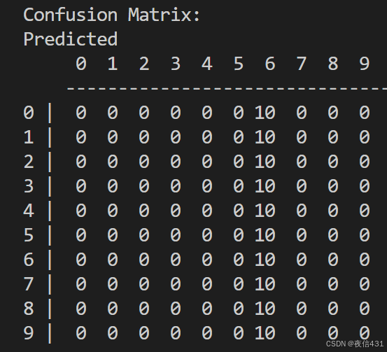

DAMO开发者矩阵,由阿里巴巴达摩院和中国互联网协会联合发起,致力于探讨最前沿的技术趋势与应用成果,搭建高质量的交流与分享平台,推动技术创新与产业应用链接,围绕“人工智能与新型计算”构建开放共享的开发者生态。
更多推荐
 20
20 0
0- 0


 已为社区贡献3条内容

所有评论(0)