今天给大家介绍机器学习中必会的 10 大机器学习算法。

1.线性回归

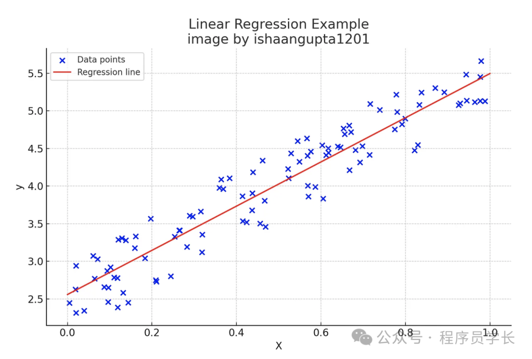
线性回归（Linear Regression）是最基本的回归分析方法之一，旨在通过线性模型来描述因变量（目标变量）与自变量（特征变量）之间的关系。

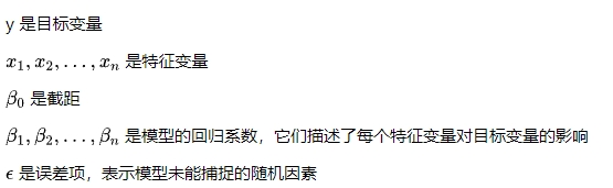
线性回归假设目标变量 y 与特征变量 X 之间呈现线性关系，模型公式为：

其中：

图片

线性回归的目标是找到最优的回归系数 ，使得预测值与实际值之间的差异最小。

复制

• .

2.逻辑回归

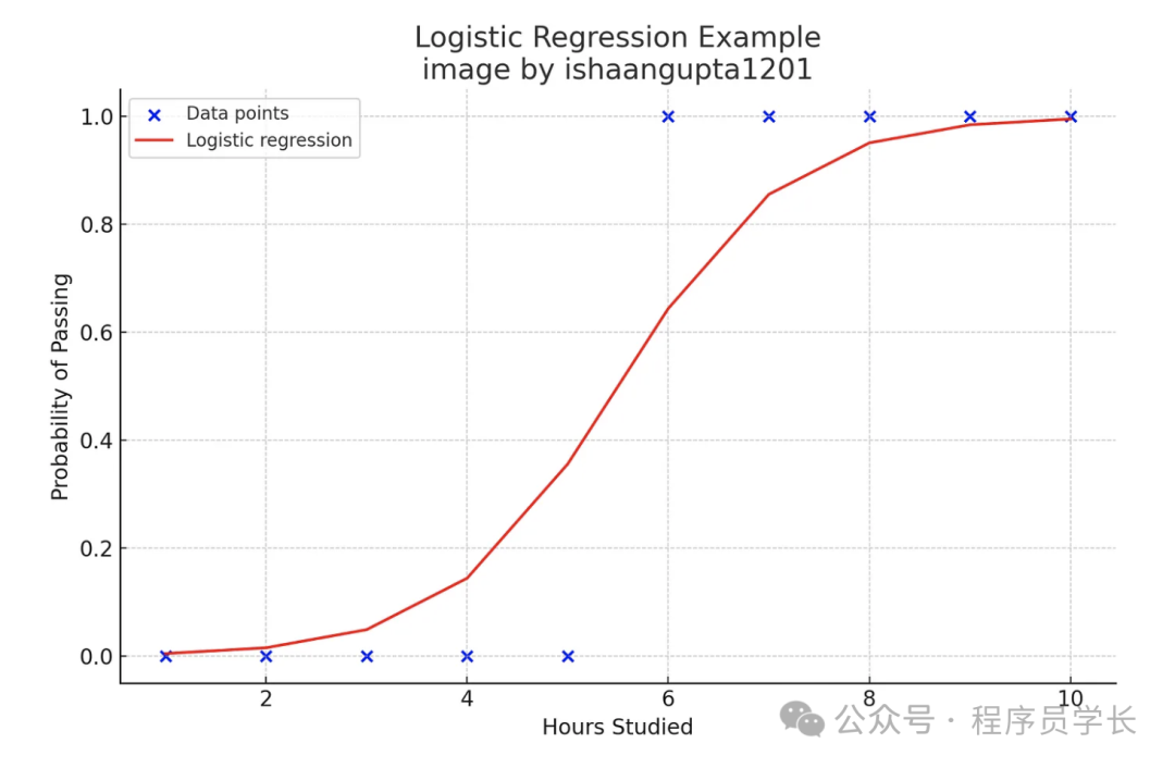
逻辑回归（Logistic Regression）虽然带有“回归”之名，但其实是一种广义线性模型，常用于二分类问题。

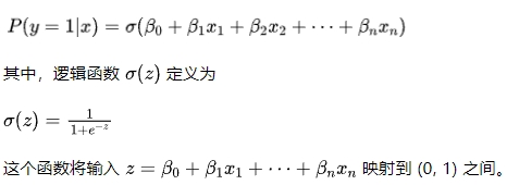
逻辑回归的核心思想是通过逻辑函数（Logistic Function），将线性回归模型的输出映射到区间 (0, 1) 上，来表示事件发生的概率。

对于一个给定的输入特征 x，模型预测为：

图片

复制

import numpy as np
from sklearn.linear_model import LogisticRegression

# Sample data: hours studied and pass/fail outcome
hours_studied = np.array([1, 2, 3, 4, 5, 6, 7, 8, 9, 10]).reshape(-1, 1)
outcome = np.array([0, 0, 0, 0, 0, 1, 1, 1, 1, 1])

# Create and train the model
model = LogisticRegression()
model.fit(hours_studied, outcome)

# This results in an array of predicted binary outcomes (0 or 1).
predicted_outcome = model.predict(hours_studied)

# This results in an array where each sub-array contains two probabilities: the probability of failing and the probability of passing.
predicted_probabilities = model.predict_proba(hours_studied)

print("Predicted Outcomes:", predicted_outcome)
print("Predicted Probabilities:", predicted_probabilities)

3. 决策树

决策树是一种基于树结构的监督学习算法，可用于分类和回归任务。

决策树模型由节点和边组成，每个节点表示一个特征或决策，边代表根据特征值分裂数据的方式。树的叶子节点对应最终的预测结果。

决策树通过递归地选择最佳的特征进行分裂，直到所有数据被准确分类或满足某些停止条件。常用的分裂标准包括信息增益（Information Gain）和基尼指数（Gini Index）。

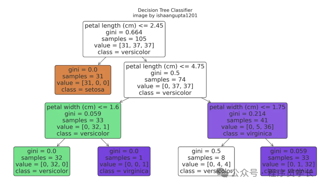
图片

复制

from sklearn.tree import DecisionTreeClassifier, plot_tree
from sklearn.datasets import load_iris
from sklearn.model_selection import train_test_split
from sklearn.metrics import accuracy_score, classification_report

# Load the iris dataset
iris = load_iris()
X, y = iris.data, iris.target

# splits the data into training and testing sets. 30% of the data is used for testing (test_size=0.3), and the rest for training. random_state=42 ensures the split is reproducible.
X_train, X_test, y_train, y_test = train_test_split(X, y, test_size=0.3, random_state=42)

# creates a decision tree classifier with a maximum depth of 3 levels and a fixed random state for reproducibility.
model = DecisionTreeClassifier(max_depth=3, random_state=42)
model.fit(X_train, y_train)

# Make predictions
y_pred = model.predict(X_test)

# Evaluate the model
accuracy = accuracy_score(y_test, y_pred)  #calculates the accuracy of the model’s predictions.
print(f"Accuracy: {accuracy:.2f}")
print("\nClassification Report:")
print(classification_report(y_test, y_pred, target_names=iris.target_names))

# Visualize the tree
plt.figure(figsize=(20,10))
plot_tree(model, feature_names=iris.feature_names, class_names=iris.target_names, filled=True, rounded=True)
plt.show()

4.支持向量机

支持向量机 (SVM) 是一种监督学习算法，可用于分类或回归问题。

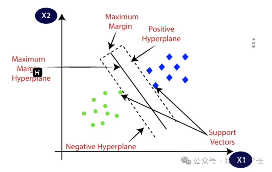
SVM 的核心思想是找到一个超平面，将数据点分成不同的类，并且这个超平面能够最大化两类数据点之间的间隔（Margin）。

超平面

超平面是一个能够将不同类别的数据点分开的决策边界。

在二维空间中，超平面就是一条直线；在三维空间中，超平面是一个平面；而在更高维空间中，超平面是一个维度比空间低一维的几何对象。

形式上，在 n 维空间中，超平面可以表示为。

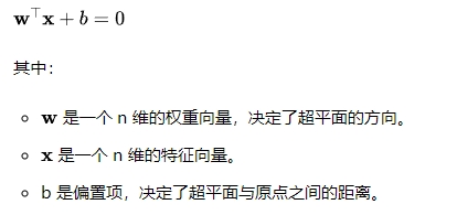
在 SVM 中，超平面用于将不同类别的数据点分开，即将正类数据点与负类数据点分隔开。

支持向量

支持向量是指在分类问题中，距离超平面最近的数据点。

这些点在 SVM 中起着关键作用，因为它们直接影响到超平面的位置和方向。

间隔

间隔（Margin）是指超平面到最近的支持向量的距离。

最大间隔

最大间隔是指支持向量机在寻找超平面的过程中，选择能够使正类和负类数据点之间的间隔最大化的那个超平面。

图片

复制

from sklearn.datasets import load_wine
from sklearn.svm import SVC
from sklearn.model_selection import train_test_split

# Load the wine dataset
X, y = load_wine(return_X_y=True)

# Split the data into training and testing sets
X_train, X_test, y_train, y_test = train_test_split(X, y, test_size=0.2, random_state=42)

# Create and train the model
model = SVC(kernel='linear', random_state=42)
model.fit(X_train, y_train)

# Make predictions
y_pred = model.predict(X_test)

print("Predictions:", y_pred)

5.朴素贝叶斯

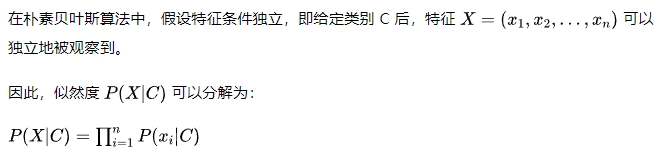
朴素贝叶斯是一种基于贝叶斯定理的简单而强大的分类算法，广泛用于文本分类、垃圾邮件过滤等问题。

其核心思想是假设所有特征之间相互独立，并通过计算每个类别的后验概率来进行分类。

贝叶斯定理定义为

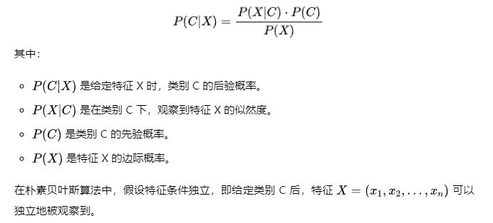
复制

from sklearn.datasets import load_digits
from sklearn.naive_bayes import GaussianNB
from sklearn.model_selection import train_test_split

# Load the digits dataset
X, y = load_digits(return_X_y=True)

# Split the data into training and testing sets
X_train, X_test, y_train, y_test = train_test_split(X, y, test_size=0.2, random_state=42)

# Create and train the model
model = GaussianNB()
model.fit(X_train, y_train)

# Make predictions
y_pred = model.predict(X_test)

print("Predictions:", y_pred)

6.KNN

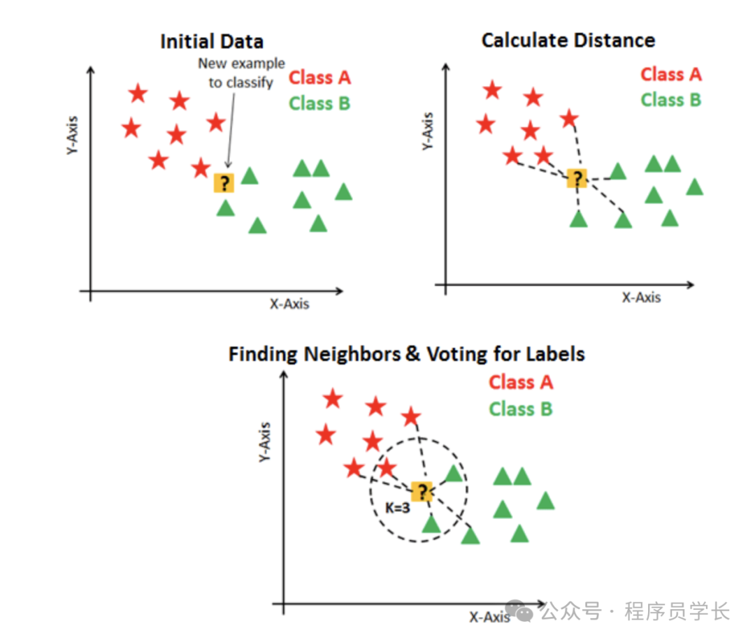
K-Nearest Neighbors (KNN) 是一种简单且直观的监督学习算法，通常用于分类和回归任务。

它的基本思想是：给定一个新的数据点，算法通过查看其最近的 K 个邻居来决定这个点所属的类别（分类）或预测其值（回归）。

KNN 不需要显式的训练过程，而是直接在预测时利用整个训练数据集。

图片

算法步骤

• 步骤1
  选择参数 K，即最近邻居的数量。
• 步骤2
  计算新数据点与训练数据集中所有点之间的距离。
  常用的距离度量包括欧氏距离、曼哈顿距离、切比雪夫距离等。
• 步骤3
  根据计算出的距离，找出距离最近的 K 个点。
• 步骤4
  对于分类问题，通过对这 K 个点的类别进行投票，选择得票最多的类别作为新数据点的预测类别。
  对于回归问题，计算这 K 个点的平均值，作为新数据点的预测值。
• 步骤5
  返回预测结果。

复制

from sklearn.datasets import load_iris
from sklearn.neighbors import KNeighborsClassifier
from sklearn.model_selection import train_test_split

# Load the iris dataset
X, y = load_iris(return_X_y=True)

# Split the data into training and testing sets
X_train, X_test, y_train, y_test = train_test_split(X, y, test_size=0.2, random_state=42)

# Create and train the model
model = KNeighborsClassifier(n_neighbors=3)
model.fit(X_train, y_train)

# Make predictions
y_pred = model.predict(X_test)

print("Predictions:", y_pred)

7.K-Means

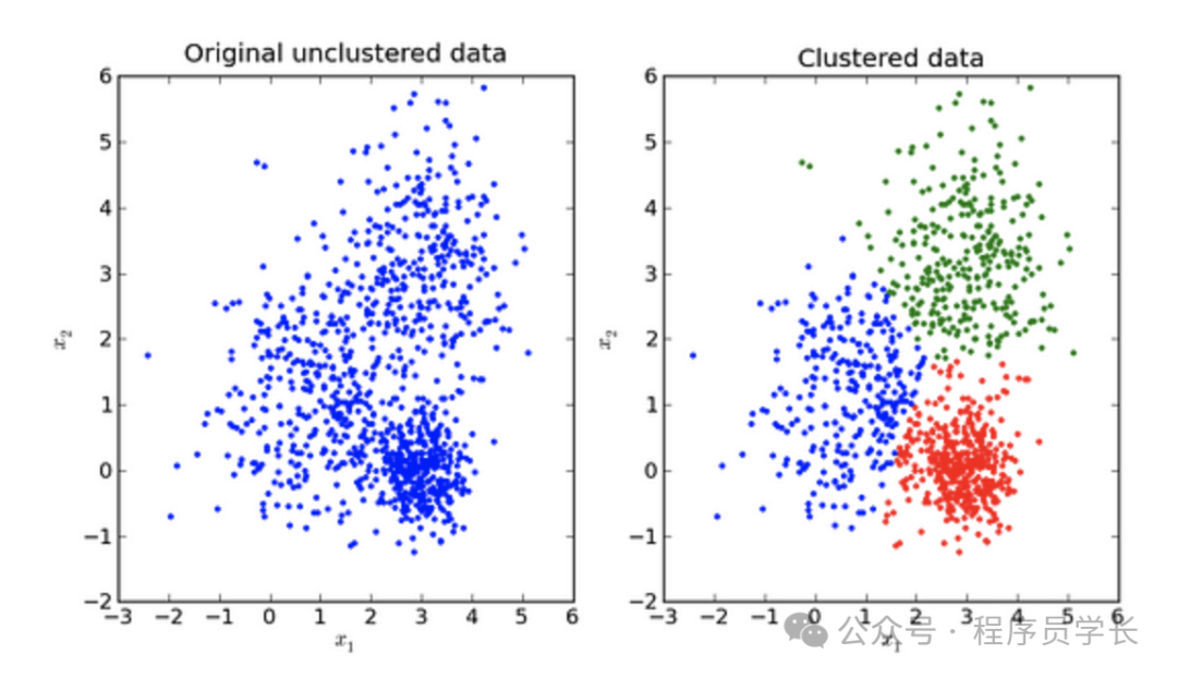
K-Means 是一种流行的无监督学习算法，主要用于聚类分析。

它的目标是将数据集分成 K 个簇，使得每个簇中的数据点与簇中心的距离最小。

算法通过迭代优化来达到最优的聚类效果。

图片

算法步骤

• 步骤1
  初始化 K 个簇中心（质心）。可以随机选择数据集中的 K 个点作为初始质心。
• 步骤2
  对于数据集中每个数据点，将其分配到与其距离最近的质心所在的簇。
• 步骤3
  重新计算每个簇的质心，即簇中所有点的平均值。
• 步骤4
  重复步骤2和步骤3，直到质心不再变化或变化量小于设定的阈值。

复制

from sklearn.datasets import make_blobs
from sklearn.cluster import KMeans

# Create a synthetic dataset
X, _ = make_blobs(n_samples=100, centers=3, n_features=2, random_state=42)

# Create and train the model
model = KMeans(n_clusters=3, random_state=42)
model.fit(X)

# Predict the clusters
labels = model.predict(X)

print("Cluster labels:", labels)

8.随机森林

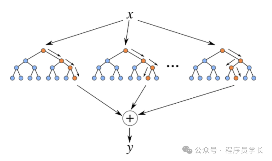
随机森林 (Random Forest) 是一种集成学习方法，主要用于分类和回归任务。

它通过结合多个决策树的预测结果来提高模型的泛化能力和鲁棒性。

随机森林的核心思想是通过引入随机性来构建多个不同的决策树模型，然后对这些模型的预测结果进行投票或平均，从而获得最终的预测结果。

图片

算法步骤

• 步骤1
  从训练数据集中随机抽取多个子样本（使用有放回的抽样方法，即Bootstrap抽样），每个子样本用于训练一个决策树。
• 步骤2
  对于每个决策树，在构建过程中，节点的划分使用随机选择的一部分特征，而不是全部特征。
• 步骤3
  每棵树独立生长，直到其无法进一步分裂，或者达到了某个预设的停止条件（如树的最大深度）。
• 步骤4
  对于分类任务，最终的预测结果由所有树的投票结果决定（多数投票法）；对于回归任务，预测结果为所有树的预测值的平均值。

复制

from sklearn.datasets import load_breast_cancer
from sklearn.ensemble import RandomForestClassifier
from sklearn.model_selection import train_test_split

# Load the breast cancer dataset
X, y = load_breast_cancer(return_X_y=True)

# Split the data into training and testing sets
X_train, X_test, y_train, y_test = train_test_split(X, y, test_size=0.2, random_state=42)

# Create and train the model
model = RandomForestClassifier(random_state=42)
model.fit(X_train, y_train)

# Make predictions
y_pred = model.predict(X_test)

print("Predictions:", y_pred)

9.PCA

主成分分析 (PCA) 是一种用于数据降维的统计技术。

其主要目的是通过将数据从高维空间映射到一个低维空间中，保留尽可能多的原始数据的方差。

这对于数据预处理和可视化非常有用，尤其是在处理具有大量特征的数据集时。

PCA 的核心思想是找到数据中的“主成分”（即那些方差最大且相互正交的方向），并沿着这些方向投影数据，从而降低数据的维度。

通过这种方式，PCA 可以在减少数据维度的同时尽可能保留数据的整体信息。

复制

from sklearn.datasets import load_digits
from sklearn.decomposition import PCA

# Load the digits dataset
X, y = load_digits(return_X_y=True)

# Apply PCA to reduce the number of features
pca = PCA(n_compnotallow=2)
X_reduced = pca.fit_transform(X)

print("Reduced feature set shape:", X_reduced.shape)

10.xgboost

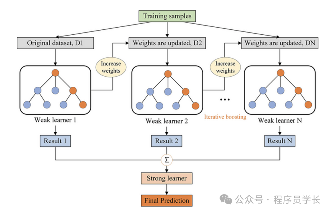
XGBoost（Extreme Gradient Boosting）是一种基于梯度提升框架的高效、灵活的机器学习算法。

它是梯度提升决策树 (GBDT) 的一种实现，具有更高的性能和更好的可扩展性，常被用来处理结构化或表格数据，并在各种数据竞赛中表现优异。

XGBoost 的核心思想是通过迭代构建多个决策树，每个新树都尝试纠正前一个树的误差。最终的预测结果是所有树的预测结果的加权和。

图片

复制

import xgboost as xgb
from sklearn.datasets import load_breast_cancer
from sklearn.model_selection import train_test_split

# Load the breast cancer dataset
X, y = load_breast_cancer(return_X_y=True)

# Split the data into training and testing sets
X_train, X_test, y_train, y_test = train_test_split(X, y, test_size=0.2, random_state=42)

# Create and train the model
model = xgb.XGBClassifier(random_state=42)
model.fit(X_train, y_train)

# Make predictions
y_pred = model.predict(X_test)

print("Predictions:", y_pred)