介绍

1.一元线性回归

在本练习的这一部分中，您将使用一个变量来实现线性回归，以预测食品车的利润。 假设你是一家特许经营餐厅的首席执行官，正在考虑在不同的城市开设新的分店。 该连锁店已经在各个城市有了卡车，而且你有了这些城市的利润和人口数据。
您希望使用这些数据来帮助您选择下一个要扩展到的城市。
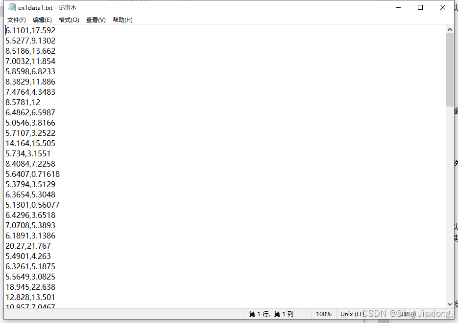
文件ex1data1.txt包含用于线性回归问题的数据集。 第一列是一个城市的人口，第二列是该城市一辆快餐车的利润。 利润为负值表示亏损。

（1）数据概览

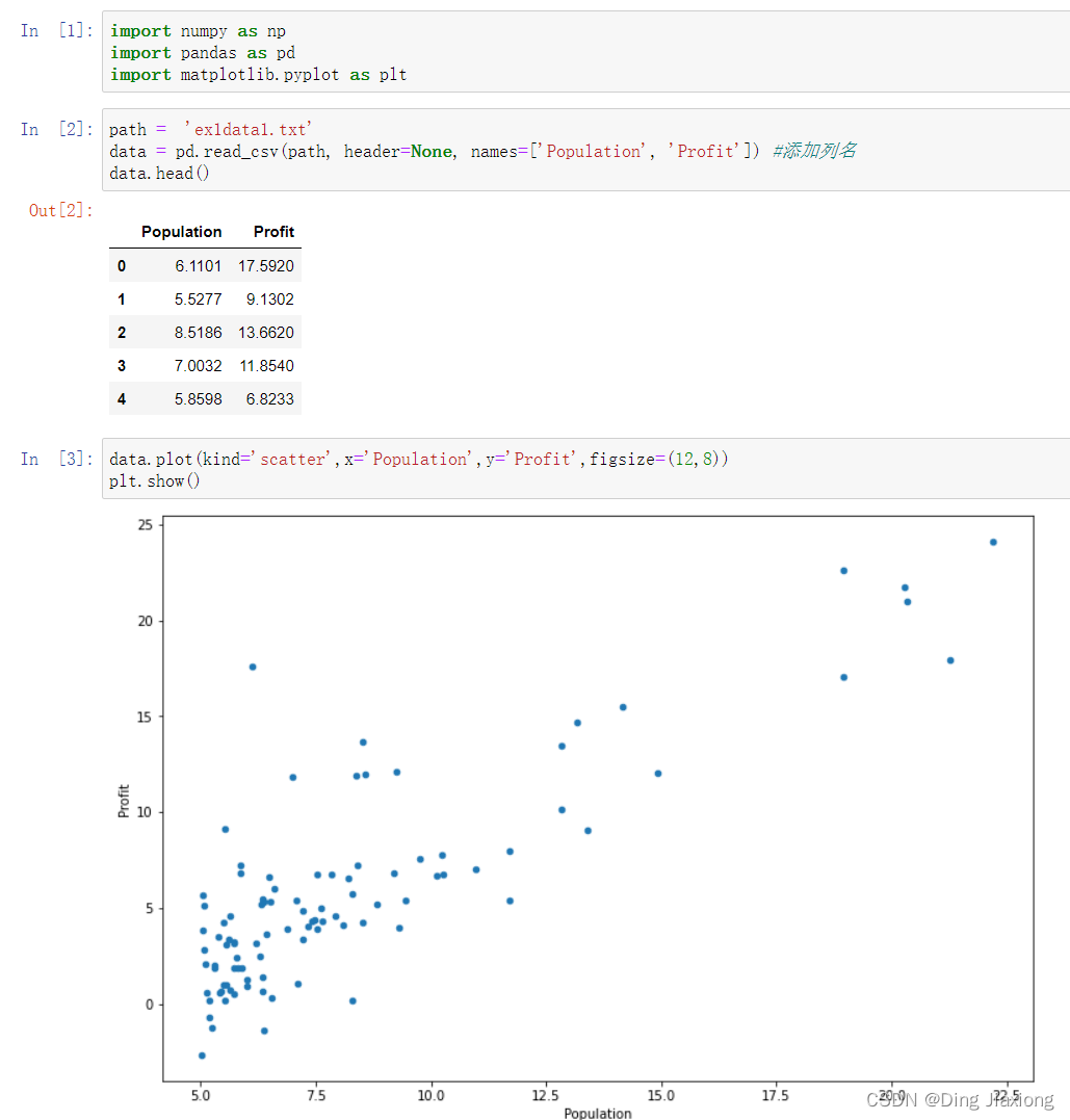
（2）绘制数据

（3）创建代价函数

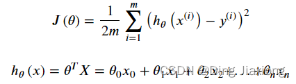
#创建代价函数
def computeCost(X, y, theta):
    inner = np.power(((X * theta.T) - y), 2)
    return np.sum(inner) / (2 * len(X))

（4）训练集中添加一列1，以便使用向量化方法计算代价以及梯度。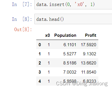

（5）特征变量X为数据的前两列，预测值(标签)为y，为数据的最后一列。

cols = data.shape[1] #cols保存的列数
X = data.iloc[:,0:cols-1]#X是所有行，去掉最后一列 左闭右开，[0,2)
y = data.iloc[:,cols-1:cols]#X是所有行，最后一列

（6）将X和y转换为numpy矩阵，并初始化theta模型参数为[0,0]

X = np.matrix(X.values)
y = np.matrix(y.values)
theta = np.matrix(np.array([0,0]))

（7）计算一下代价函数的值。此时模型参数均为0。

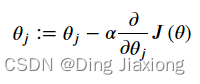
（8）创建批量梯度下降函数。

公式：

def gradientDescent(X, y, theta, alpha, iters):
    temp = np.matrix(np.zeros(theta.shape))
    parameters = int(theta.ravel().shape[1]) 
    cost = np.zeros(iters)
    
    for i in range(iters):
        error = (X * theta.T) - y
        
        for j in range(parameters):
            term = np.multiply(error, X[:,j])
            temp[0,j] = theta[0,j] - ((alpha / len(X)) * np.sum(term))
            
        theta = temp
        cost[i] = computeCost(X, y, theta)
        
    return theta, cost

（9）初始化学习率α和迭代次数。

alpha = 0.01
iters = 1000

（10）开始训练，最终输出训练完成的模型参数。

（11）使用训练出的模型参数g再次计算代价函数

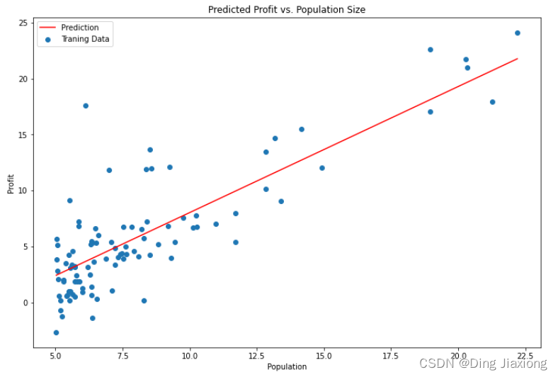
（12）绘制线性模型观察拟合数据情况。

x = np.linspace(data.Population.min(), data.Population.max(), 100)
f = g[0, 0] + (g[0, 1] * x)

fig, ax = plt.subplots(figsize=(12,8))
ax.plot(x, f, 'r', label='Prediction')
ax.scatter(data.Population, data.Profit, label='Traning Data')
ax.legend(loc=2)
ax.set_xlabel('Population')
ax.set_ylabel('Profit')
ax.set_title('Predicted Profit vs. Population Size')
plt.show()

（13）绘制代价函数计算值的变化情况。

fig, ax = plt.subplots(figsize=(12,8))
ax.plot(np.arange(iters), cost, 'r')
ax.set_xlabel('Iterations')
ax.set_ylabel('Cost')
ax.set_title('Error vs. Training Epoch')
plt.show()

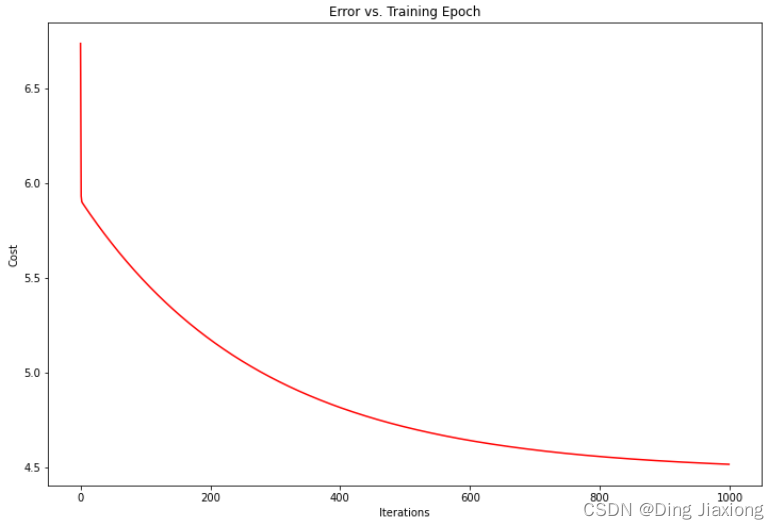
可以看出经过不断梯度下降，代价函数值越来越小，最终达到一个全局最优点。

2.多元线性回归

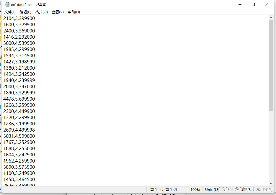
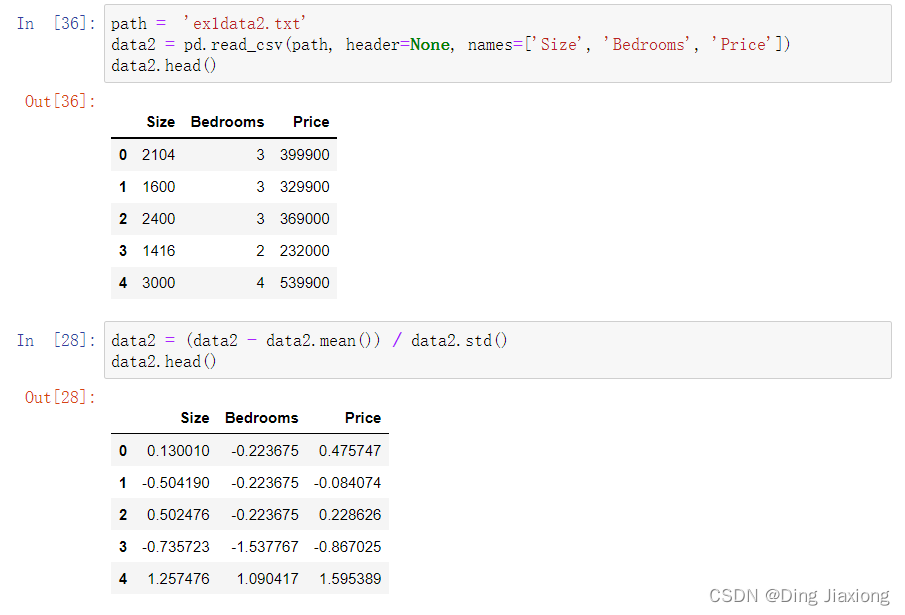
文件ex1data2.txt包含俄勒冈州Port- land房价的训练集。 第一栏是房子的大小(平方英尺)，第二栏是卧室的数量，第三栏是房子的价格。

（1）数据概览

（2）特征归一化。
在数据集中减去每个特征的平均值，并除以各自的标准差。

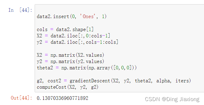
（3）数据预处理，添加一列1、初始化三个模型参数等。

data2.insert(0, 'Ones', 1)

cols = data2.shape[1]
X2 = data2.iloc[:,0:cols-1]
y2 = data2.iloc[:,cols-1:cols]

X2 = np.matrix(X2.values)
y2 = np.matrix(y2.values)
theta2 = np.matrix(np.array([0,0,0]))

g2, cost2 = gradientDescent(X2, y2, theta2, alpha, iters)
computeCost(X2, y2, g2)

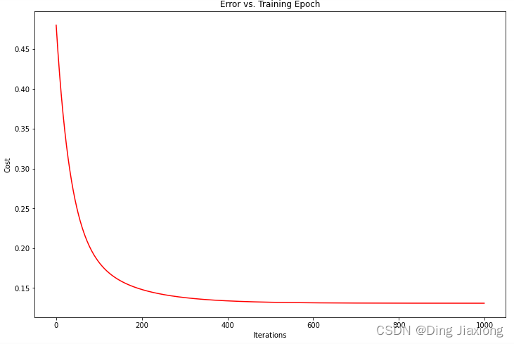
（4）观察代价函数变化。

fig, ax = plt.subplots(figsize=(12,8))
ax.plot(np.arange(iters), cost2, 'r')
ax.set_xlabel('Iterations')
ax.set_ylabel('Cost')
ax.set_title('Error vs. Training Epoch')
plt.show()

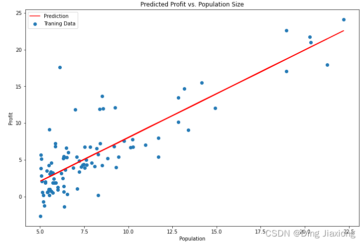
3.使用sklearn机器学习库中的线性回归函数实现第一个问题

from sklearn import linear_model
model = linear_model.LinearRegression()
model.fit(X, y)

x = np.array(X[:, 1].A1)
f = model.predict(X).flatten()

fig, ax = plt.subplots(figsize=(12,8))
ax.plot(x, f, 'r', label='Prediction')
ax.scatter(data.Population, data.Profit, label='Traning Data')
ax.legend(loc=2)
ax.set_xlabel('Population')
ax.set_ylabel('Profit')
ax.set_title('Predicted Profit vs. Population Size')
plt.show()

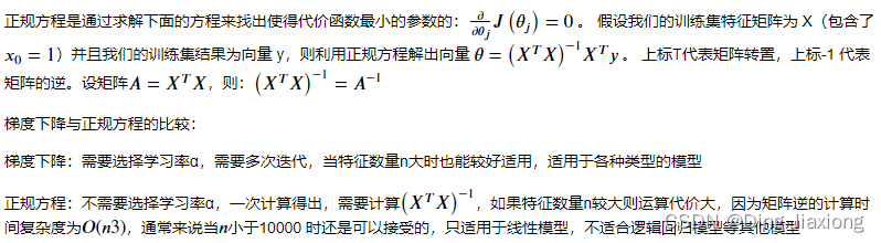
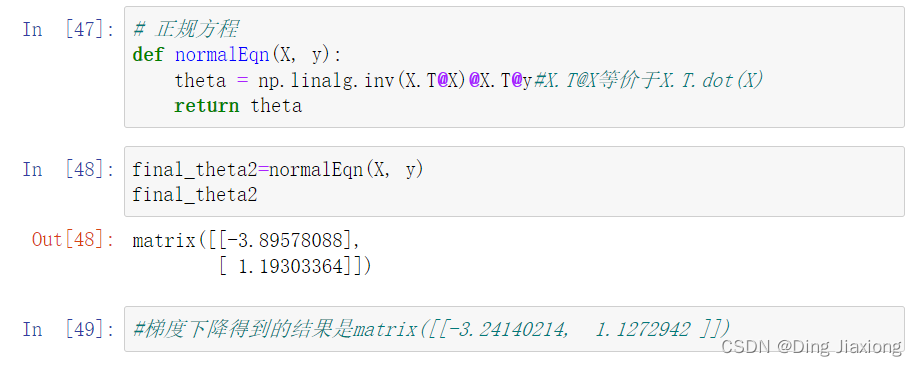
4.使用正规方程直接计算出模型参数。