单细胞Marker计算与可视化的pseudo-bulk方案

Biomamba生信基地

217人浏览 · 2026-03-10 15:56:36

Biomamba生信基地 · 2026-03-10 15:56:36 发布

一、写在前面

pseudo-bulk：把同一个细胞类型/同一群细胞的多个单细胞表达量直接相加/求和，合成一个 “虚拟的bulk样本”。也许你会有疑惑，我们花这么多钱测得单细胞，不就是为了获得单细胞分辨率的转录组数据吗？为何还要将其再合并模拟生成bulk数据？

这其实为了解决单细胞稀疏性的问题，pseudo-bulk对scRNA-seq数据求和后，信号变强、噪声被平均掉。并且在scRNA-seq进行差异分析时，细胞之间不是独立样本，所以会干扰差异分析的准确度，从而产生假阳性。故差异基因更可靠、更接近真实生物学。

此前我们演示过pseudo bulk差异分析，接下来只需要转换一下变量，即可基于scRNA‑seq数据实现不同细胞类型间的pseudo bulk标记基因计算。

本教程基于Linux环境的rstudio演示，计算资源不足的同学可参考：

足够支持你完成硕博生涯的生信环境

忘记宣传了，独享用户连技术支持都是独享的

访问链接：https://biomamba.xiyoucloud.net/

欢迎联系客服微信[Biomamba_zhushou]获取帮助

如果需要单细胞数据分析教学、生信热点全文复现、自测数据个性化分析辅导、常态化实验学习，欢迎联系客服微信[Biomamba_zhushou]。

二、实操流程

1、数据基本情况

# 加载R包
library(Seurat)

## Loading required package: SeuratObject

## Loading required package: sp

## 'SeuratObject' was built with package 'Matrix' 1.7.1 but the current
## version is 1.7.2; it is recomended that you reinstall 'SeuratObject' as
## the ABI for 'Matrix' may have changed

## 
## Attaching package: 'SeuratObject'

## The following objects are masked from 'package:base':
## 
##     intersect, t

library (dplyr)

## 
## Attaching package: 'dplyr'

## The following objects are masked from 'package:stats':
## 
##     filter, lag

## The following objects are masked from 'package:base':
## 
##     intersect, setdiff, setequal, union

# 读取数据：
scRNA <- readRDS('test_data/T1D_scRNA.rds')
# 这个数据包含24个样本：
levels(scRNA$sample)

## NULL

# 包含两个组别的数据：
DimPlot(scRNA,split.by = 'Group')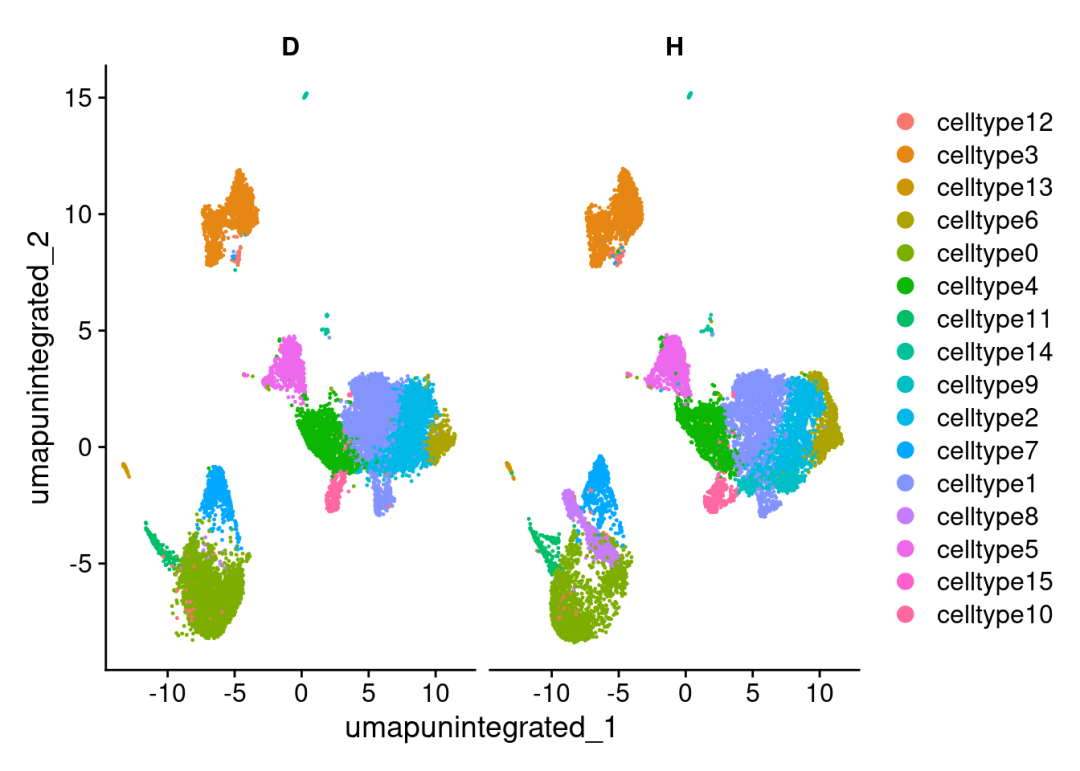

# 取五种细胞类型用于下游演示：
select_ct <- paste0('celltype',1:5)
scRNA <- scRNA[,scRNA$cell_type %in% select_ct]
DimPlot(scRNA,split.by = 'Group')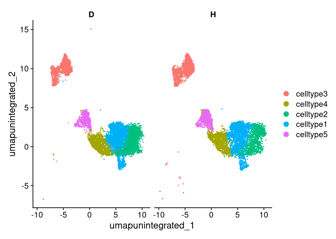

2、循环添加细胞类型专属变量

for (run_ct in select_ct) {
  target_col  <- paste0(run_ct,'_var')# 细胞类型专属变量的slot名称
  scRNA@meta.data[,target_col] <- scRNA$cell_type# 复制原始细胞变量
  scRNA@meta.data[[target_col]][scRNA@meta.data[[target_col]] %>% as.character() != run_ct] <- 'OtherS' # 除了目标细胞类型外，其它的都叫OtherS
}

3、循环生成pseudo-bulk数据并差异计算

3.1 生成拟bulk对象

bulk <- AggregateExpression(scRNA, return.seurat = T, slot = "counts", assays = "RNA",
                            group.by = c("cell_type", "sample", "Group",paste0(select_ct,'_var'))# 分别填写细胞类型、样本变量、分组变量的slot名称
    )

## Names of identity class contain underscores ('_'), replacing with dashes ('-')
## Centering and scaling data matrix
## 
## This message is displayed once every 8 hours.

# 生成的是一个新的Seurat对象：
bulk

## An object of class Seurat 
## 41056 features across 120 samples within 1 assay 
## Active assay: RNA (41056 features, 0 variable features)
##  3 layers present: counts, data, scale.data

3.2 pseudo-bulk计算细胞marker

# 差异分析会用到bulk分析常用到的DESeq2：
if(!require(DESeq2))BiocManager::install('DESeq2')

## Loading required package: DESeq2

## Loading required package: S4Vectors

## Loading required package: stats4

## Loading required package: BiocGenerics

## 
## Attaching package: 'BiocGenerics'

## The following objects are masked from 'package:dplyr':
## 
##     combine, intersect, setdiff, union

## The following object is masked from 'package:SeuratObject':
## 
##     intersect

## The following objects are masked from 'package:stats':
## 
##     IQR, mad, sd, var, xtabs

## The following objects are masked from 'package:base':
## 
##     anyDuplicated, aperm, append, as.data.frame, basename, cbind,
##     colnames, dirname, do.call, duplicated, eval, evalq, Filter, Find,
##     get, grep, grepl, intersect, is.unsorted, lapply, Map, mapply,
##     match, mget, order, paste, pmax, pmax.int, pmin, pmin.int,
##     Position, rank, rbind, Reduce, rownames, sapply, saveRDS, setdiff,
##     table, tapply, union, unique, unsplit, which.max, which.min

## 
## Attaching package: 'S4Vectors'

## The following objects are masked from 'package:dplyr':
## 
##     first, rename

## The following object is masked from 'package:utils':
## 
##     findMatches

## The following objects are masked from 'package:base':
## 
##     expand.grid, I, unname

## Loading required package: IRanges

## 
## Attaching package: 'IRanges'

## The following objects are masked from 'package:dplyr':
## 
##     collapse, desc, slice

## The following object is masked from 'package:sp':
## 
##     %over%

## Loading required package: GenomicRanges

## Loading required package: GenomeInfoDb

## Loading required package: SummarizedExperiment

## Loading required package: MatrixGenerics

## Loading required package: matrixStats

## 
## Attaching package: 'matrixStats'

## The following object is masked from 'package:dplyr':
## 
##     count

## 
## Attaching package: 'MatrixGenerics'

## The following objects are masked from 'package:matrixStats':
## 
##     colAlls, colAnyNAs, colAnys, colAvgsPerRowSet, colCollapse,
##     colCounts, colCummaxs, colCummins, colCumprods, colCumsums,
##     colDiffs, colIQRDiffs, colIQRs, colLogSumExps, colMadDiffs,
##     colMads, colMaxs, colMeans2, colMedians, colMins, colOrderStats,
##     colProds, colQuantiles, colRanges, colRanks, colSdDiffs, colSds,
##     colSums2, colTabulates, colVarDiffs, colVars, colWeightedMads,
##     colWeightedMeans, colWeightedMedians, colWeightedSds,
##     colWeightedVars, rowAlls, rowAnyNAs, rowAnys, rowAvgsPerColSet,
##     rowCollapse, rowCounts, rowCummaxs, rowCummins, rowCumprods,
##     rowCumsums, rowDiffs, rowIQRDiffs, rowIQRs, rowLogSumExps,
##     rowMadDiffs, rowMads, rowMaxs, rowMeans2, rowMedians, rowMins,
##     rowOrderStats, rowProds, rowQuantiles, rowRanges, rowRanks,
##     rowSdDiffs, rowSds, rowSums2, rowTabulates, rowVarDiffs, rowVars,
##     rowWeightedMads, rowWeightedMeans, rowWeightedMedians,
##     rowWeightedSds, rowWeightedVars

## Loading required package: Biobase

## Welcome to Bioconductor
## 
##     Vignettes contain introductory material; view with
##     'browseVignettes()'. To cite Bioconductor, see
##     'citation("Biobase")', and for packages 'citation("pkgname")'.

## 
## Attaching package: 'Biobase'

## The following object is masked from 'package:MatrixGenerics':
## 
##     rowMedians

## The following objects are masked from 'package:matrixStats':
## 
##     anyMissing, rowMedians

## 
## Attaching package: 'SummarizedExperiment'

## The following object is masked from 'package:Seurat':
## 
##     Assays

## The following object is masked from 'package:SeuratObject':
## 
##     Assays

# 创建空的数据框
mk_df <- data.frame()
for (run_ct in select_ct) {
  # 改变默认分类变量：
 Idents(bulk) <- paste0(run_ct,'_var')
 # 下面的计算依赖DESeq2，做过Bulk RNA-Seq的同学都知道：
bulk_deg <- FindMarkers(bulk, ident.1 = run_ct, ident.2 = "OtherS", # 这样算出来的Fold Change就是run_ct/OtherS
                          slot = "counts", test.use = "DESeq2",# 这里可以选择其它算法
      verbose = F# 关闭进度提示
      )
bulk_deg$Celltype <- run_ct# 添加一列，收录当前进行差异计算的细胞类型
bulk_deg$gene <- rownames(bulk_deg)# 添加基因列  
mk_df <- rbind(mk_df,bulk_deg)# 纵向合并数据框
}

## converting counts to integer mode

## gene-wise dispersion estimates

## mean-dispersion relationship

## final dispersion estimates

## converting counts to integer mode

## gene-wise dispersion estimates

## mean-dispersion relationship

## final dispersion estimates

## converting counts to integer mode

## gene-wise dispersion estimates

## mean-dispersion relationship

## final dispersion estimates

## converting counts to integer mode

## gene-wise dispersion estimates

## mean-dispersion relationship

## final dispersion estimates

## converting counts to integer mode

## gene-wise dispersion estimates

## mean-dispersion relationship

## final dispersion estimates

# 计算top marker
top3_mk <- mk_df %>% group_by(Celltype) %>% top_n(n = 3, wt = avg_log2FC)  
top3_mk

## # A tibble: 15 × 7
## # Groups:   Celltype [5]
##        p_val avg_log2FC pct.1 pct.2 p_val_adj Celltype  gene           
##        <dbl>      <dbl> <dbl> <dbl>     <dbl> <chr>     <chr>          
##  1 6.52e- 37       3.45 1     0.823 2.68e- 32 celltype1 ENSG00000227240
##  2 3.00e- 20       3.89 0.958   0.25  1.23e- 15 celltype1 ENSG00000041515
##  3 3.25e- 14       3.87 0.958   0.281 1.33e-  9 celltype1 ENSG00000163629
##  4 1.74e- 65       4.50 1     0.396 7.15e- 61 celltype2 ENSG00000156395
##  5 8.25e- 53       4.10 1     0.177 3.39e- 48 celltype2 ENSG00000238241
##  6 3.55e- 16       4.22 0.875   0.25  1.46e- 11 celltype2 ENSG00000158966
##  7 0            7.18 1     0.615 0      celltype3 ENSG00000144645
##  8 0            7.40 1     0.625 0       celltype3 ENSG00000196092
##  9 5.37e-116       7.18 1     0.156 2.20e-111 celltype3 ENSG00000150625
## 10 3.34e- 18        4.05 1     0.604 1.37e- 13 celltype4 ENSG00000170624
## 11 4.24e- 18        4.05 0.833   0.333 1.74e- 13 celltype4 ENSG00000276241
## 12 9.19e- 10        3.61 0.667   0.073 3.77e- 5 celltype4 ENSG00000244649
## 13 8.73e-126        6.45 1     0.229 3.58e-121 celltype5 ENSG00000165061
## 14 1.17e- 57        5.45 0.958   0.229 4.80e- 53 celltype5 ENSG00000169744
## 15 2.17e- 35        5.40 1     0.427 8.91e- 31 celltype5 ENSG00000149403

# 更改默认标签为细胞类型
Idents(bulk) <-  bulk$cell_type                               
# 小提琴图看看我们拟bulk获得的基因效果如何：
VlnPlot(bulk,top3_mk$gene,stack = T)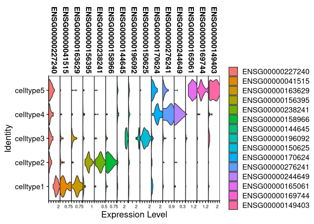

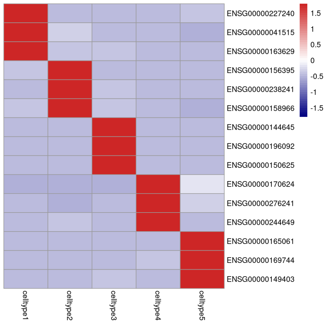
4、热图绘制

为了更有拟bulk的味道，热图也可以用平均值来绘制：

#获得表达均值矩阵：
avg <- AverageExpression(scRNA,features = top3_mk$gene)[["RNA"]]

## As of Seurat v5, we recommend using AggregateExpression to perform pseudo-bulk analysis.
## This message is displayed once per session.

avg <- as.data.frame(avg)
library(pheatmap)
# 绘制热图
pheatmap(avg[,select_ct],
         cluster_rows = F,cluster_cols = F, 
#行和列的聚类都关掉
，方便我们按顺序观察结果  
         show_colnames = T,
#展示横坐标的细胞分群
         color = colorRampPalette(c("navy", "white", "firebrick3"))(50), 
#修改渐变色
         scale = "row"
         )