1.生成模拟数据集

可以用make_classification()函数来生成模拟数据集

from sklearn.datasets import make_classification

X, y = make_classification(n_samples=1000, n_features=20, n_classes=2, random_state=42)

这里各个参数的含义分别是："n_samples"是指样本数量，"n_features"是指每个样本的特征数量，

"n_classes"是指分类的类别数，这里'n_classes=2'就是指该分类任务是一个二分类任务，"random_state"是随机种子，用于控制生成数据集的随机性。

可以用下面这段代码输出生成的数据集中的前5个数据

print('特征:',X[:5])
print('标签:',y[:5])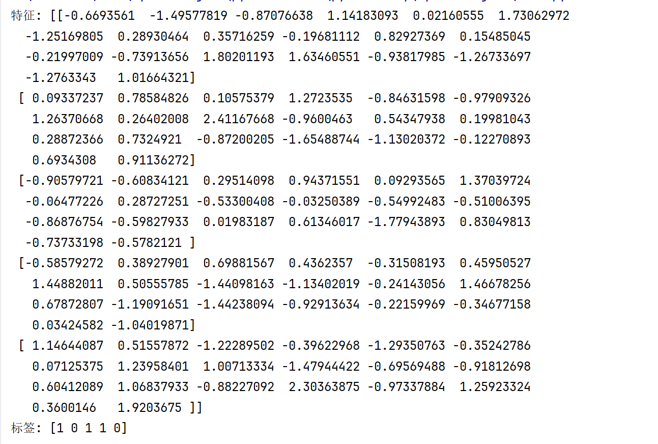

2.划分数据集并计算混淆矩阵的值

划分数据集有很多方法，比如留出法，交叉验证法等。这里我们用10折交叉验证法来划分数据集

这里我们用KFold()就可以实现交叉验证法的划分，由于我们需要绘制ROC曲线和P-R曲线，所以我们要计算这两个曲线所用的数据。并计算其对应的评估指标F1值和AUC值。

# 初始化 KFold，n_splits=10 表示 10 折交叉验证
kf = KFold(n_splits=10, shuffle=True, random_state=42)

# 初始化存储每一折的计算结果
all_confusion_matrices = []
all_precision = []
all_recall = []
all_fpr = []
all_tpr = []
all_f1_scores = []
all_auc_scores = []

# 遍历每一折，划分训练集和测试集
for train_index, test_index in kf.split(X):
    # 获取训练集和测试集
    X_train, X_test = X[train_index], X[test_index]
    y_train, y_test = y[train_index], y[test_index]

    # 创建KNN分类器，设置邻居数量为5，并进行模型训练
    knn = KNeighborsClassifier(n_neighbors=5)
    knn.fit(X_train, y_train)

    # 获取预测的概率（用于计算ROC曲线和P-R曲线）
    y_scores = knn.predict_proba(X_test)[:, 1]  # 获取类别1的预测概率

    # 获取预测标签（根据某个阈值）
    y_pred = knn.predict(X_test)

    # 计算混淆矩阵
    cm = confusion_matrix(y_test, y_pred)
    all_confusion_matrices.append(cm)

    # 计算 P-R 曲线
    precision, recall, _ = precision_recall_curve(y_test, y_scores)
    all_precision.append(precision)
    all_recall.append(recall)

    # 计算 ROC 曲线
    fpr, tpr, _ = roc_curve(y_test, y_scores)
    all_fpr.append(fpr)
    all_tpr.append(tpr)

    # 计算F1值
    f1 = f1_score(y_test, y_pred)
    all_f1_scores.append(f1)

    # 计算AUC值
    auc = roc_auc_score(y_test, y_scores)
    all_auc_scores.append(auc)

# 计算每个折的混淆矩阵平均值
average_cm = np.mean(all_confusion_matrices, axis=0)

# 计算 P-R 曲线和 ROC 曲线的平均值
mean_precision = np.mean(all_precision, axis=0)
mean_recall = np.mean(all_recall, axis=0)

# 计算ROC曲线的平均值
mean_fpr = np.linspace(0, 1, 100)
mean_tpr = np.mean([np.interp(mean_fpr, fpr, tpr) for fpr, tpr in zip(all_fpr, all_tpr)], axis=0)

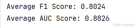
# 计算F1值和AUC值的平均值
mean_f1_score = np.mean(all_f1_scores)
mean_auc_score = np.mean(all_auc_scores)

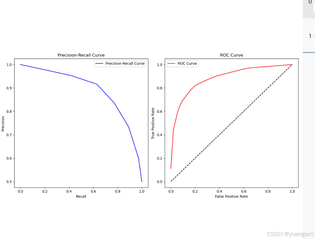
3.绘制曲线

# 绘制 P-R 曲线和 ROC 曲线
plt.figure(figsize=(12, 6))

# P-R 曲线
plt.subplot(1, 2, 1)
plt.plot(mean_recall, mean_precision, color='b', label='Precision-Recall Curve')
plt.xlabel('Recall')
plt.ylabel('Precision')
plt.title('Precision-Recall Curve')
plt.legend(loc='best')

# ROC 曲线
plt.subplot(1, 2, 2)
plt.plot(mean_fpr, mean_tpr, color='r', label='ROC Curve')
plt.plot([0, 1], [0, 1], color='black', linestyle='--')  # 随机猜测的基准线
plt.xlabel('False Positive Rate')
plt.ylabel('True Positive Rate')
plt.title('ROC Curve')
plt.legend(loc='best')

plt.tight_layout()
plt.show()

实验结果如下

实验过程中遇到的问题和错误

这里我对交叉验证法产生了误解，因为绘制P-R曲线和ROC曲线需要多个混淆矩阵得到多个点来连线，但是10折交叉验证法不是用来得到多个混淆矩阵的方法，正确的方法应该是改变判断阈值，导致我的曲线绘制如下

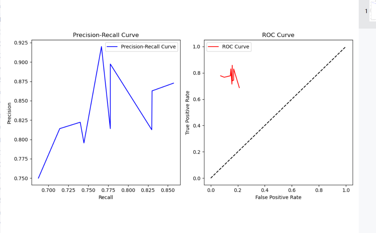
这并不符合预期的结果，因为ROC曲线的性能评价指标就是与对角线围成的面积。