结构优化设计-主题066-基于机器学习的拓扑优化

kkchenkx

315人浏览 · 2026-04-19 12:07:28

kkchenkx · 2026-04-19 12:07:28 发布

主题066：基于机器学习的拓扑优化

一、场景描述

核心问题：传统拓扑优化（如SIMP方法）虽然能够获得高质量的结构设计，但需要进行数十次甚至上百次的有限元分析迭代，计算成本高昂。在概念设计阶段需要快速探索大量设计方案时，或在需要实时交互式优化的应用场景中，传统方法难以满足效率要求。

机器学习解决方案：通过训练神经网络代理模型，学习从设计参数到最优拓扑结构的映射关系，实现单次前向传播即可预测最优拓扑，将计算时间从分钟级缩短到毫秒级，加速比可达100-1000倍。

在这里插入图片描述

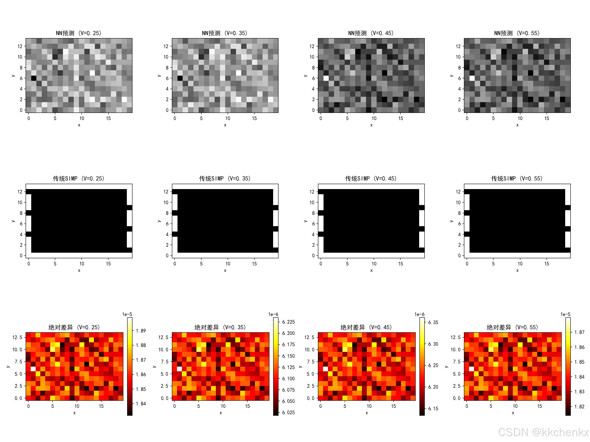
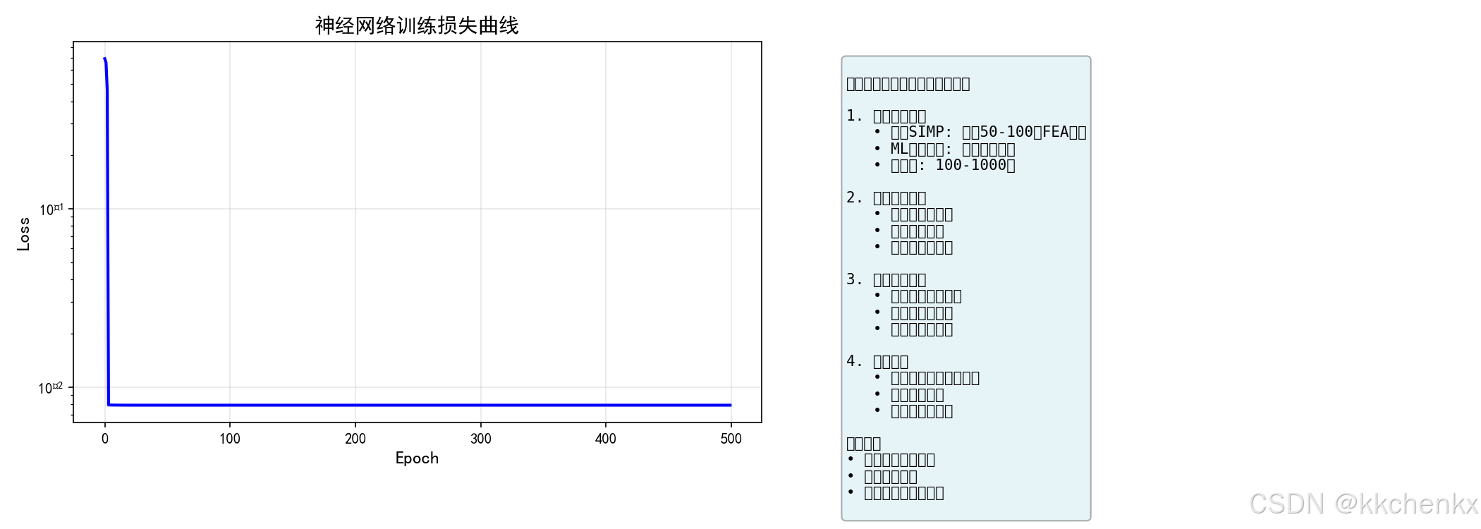
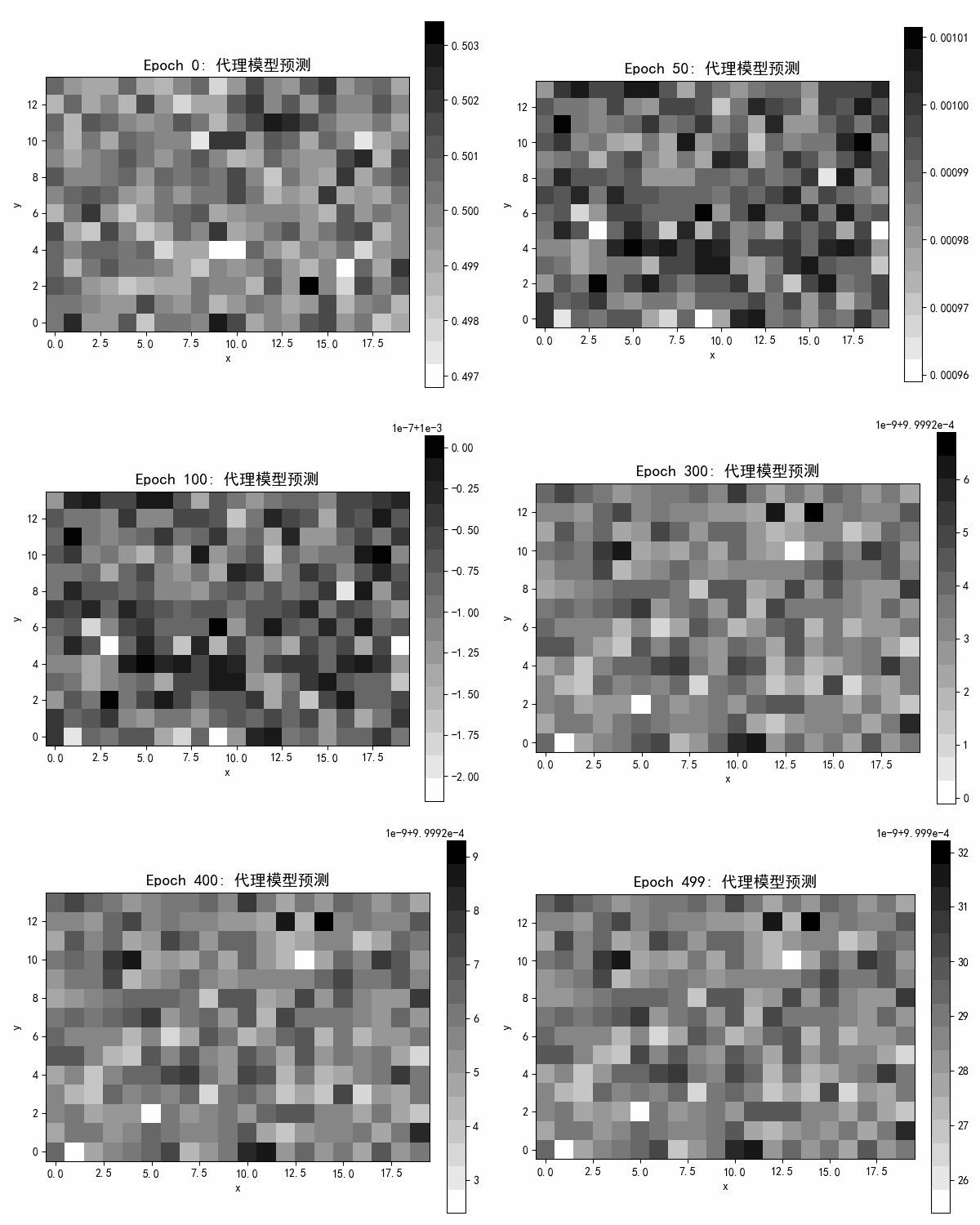
二、数学与物理模型

2.1 问题表述

传统拓扑优化的数学表述：

$\begin{aligned} \min_{\rho} \quad & c(\rho) = \mathbf{F}^T \mathbf{U} \\ \text{s.t.} \quad & \mathbf{K}(\rho) \mathbf{U} = \mathbf{F} \\ & \frac{1}{|\Omega|} \int_\Omega \rho \, d\Omega \leq V^* \\ & 0 < \rho_{\min} \leq \rho \leq 1 \end{aligned}$

其中 $ρ\rho$ 是单元密度场， $c$ 是结构柔度， $V^*$ 是体积约束上限。

2.2 机器学习视角

将拓扑优化视为一个函数逼近问题：

$\rho^* = f(\mathbf{x}; \theta)$

其中：

$x\mathbf{x}$ ：输入特征（边界条件、载荷、体积分数等）
$ρ∗\rho^*$ ：最优密度场
$θ\theta$ ：神经网络参数
$f$ ：神经网络映射函数

2.3 神经网络架构

采用全连接神经网络：

$z[1]=W[1]x+b[1]a[1]=ReLU(z[1])z[2]=W[2]a[1]+b[2]ρ^=σ(z[2]) \begin{aligned} \mathbf{z}^{[1]} &= \mathbf{W}^{[1]} \mathbf{x} + \mathbf{b}^{[1]} \\ \mathbf{a}^{[1]} &= \text{ReLU}(\mathbf{z}^{[1]}) \\ \mathbf{z}^{[2]} &= \mathbf{W}^{[2]} \mathbf{a}^{[1]} + \mathbf{b}^{[2]} \\ \hat{\rho} &= \sigma(\mathbf{z}^{[2]}) \end{aligned}$

损失函数采用二元交叉熵：

$L=−1N∑i=1N[ρilog⁡(ρ^i)+(1−ρi)log⁡(1−ρ^i)] \mathcal{L} = -\frac{1}{N} \sum_{i=1}^{N} \left[ \rho_i \log(\hat{\rho}_i) + (1-\rho_i) \log(1-\hat{\rho}_i) \right]$

三、环境准备

# 基础依赖
pip install numpy matplotlib pillow

# 可选：使用PyTorch/TensorFlow构建更复杂的模型
pip install torch torchvision

四、完整代码实现

# -*- coding: utf-8 -*-
"""
主题066：基于机器学习的拓扑优化
案例：使用神经网络代理模型加速拓扑优化
"""

import numpy as np
import matplotlib
matplotlib.use('Agg')
import matplotlib.pyplot as plt
from matplotlib.colors import LinearSegmentedColormap
import warnings
warnings.filterwarnings('ignore')
import os
from PIL import Image

# 创建输出目录
output_dir = r'd:\文档\500仿真领域\工程仿真\结构优化设计\主题066'
os.makedirs(output_dir, exist_ok=True)

plt.rcParams['font.sans-serif'] = ['SimHei', 'DejaVu Sans', 'Arial Unicode MS']
plt.rcParams['axes.unicode_minus'] = False

print("=" * 80)
print("基于机器学习的拓扑优化 - 神经网络代理模型")
print("=" * 80)

# ==================== 1. 传统拓扑优化实现（用于生成训练数据）====================
def traditional_topology_optimization(nelx, nely, volfrac, max_iter=50):
    """
    传统SIMP拓扑优化（用于生成训练数据）
    """
    E0, Emin, penal = 1.0, 1e-9, 3.0
    
    # 初始化
    x = np.ones(nelx * nely) * volfrac
    xPhys = x.copy()
    
    # 有限元准备
    def lk():
        k = np.array([
            [ 0.5,  0.0,  0.0,  0.0, -0.5,  0.0,  0.0,  0.0],
            [ 0.0,  0.5,  0.0,  0.0,  0.0, -0.5,  0.0,  0.0],
            [ 0.0,  0.0,  0.5,  0.0,  0.0,  0.0, -0.5,  0.0],
            [ 0.0,  0.0,  0.0,  0.5,  0.0,  0.0,  0.0, -0.5],
            [-0.5,  0.0,  0.0,  0.0,  0.5,  0.0,  0.0,  0.0],
            [ 0.0, -0.5,  0.0,  0.0,  0.0,  0.5,  0.0,  0.0],
            [ 0.0,  0.0, -0.5,  0.0,  0.0,  0.0,  0.5,  0.0],
            [ 0.0,  0.0,  0.0, -0.5,  0.0,  0.0,  0.0,  0.5]
        ])
        return k
    
    KE = lk()
    nElements = nelx * nely
    nNodes = (nelx + 1) * (nely + 1)
    nDOF = 2 * nNodes
    
    # 载荷与边界条件（悬臂梁）
    F = np.zeros(nDOF)
    F[1] = -1.0  # 左上角加载
    
    fixed_dofs = []
    for i in range(nely + 1):
        node = i
        fixed_dofs.extend([2 * node, 2 * node + 1])
    free_dofs = np.setdiff1d(np.arange(nDOF), fixed_dofs)
    
    # 过滤矩阵
    rmin = 1.5
    H = np.zeros((nElements, nElements))
    for i in range(nelx):
        for j in range(nely):
            el1 = i * nely + j
            for k in range(max(0, i-int(rmin)), min(nelx, i+int(rmin)+1)):
                for l in range(max(0, j-int(rmin)), min(nely, j+int(rmin)+1)):
                    el2 = k * nely + l
                    dist = np.sqrt((i-k)**2 + (j-l)**2)
                    if dist <= rmin:
                        H[el1, el2] = rmin - dist
    Hs = np.sum(H, axis=1)
    
    # 自由度映射
    def edofRow(nelx, nely):
        edofMat = np.zeros((nElements, 8), dtype=int)
        for elx in range(nelx):
            for ely in range(nely):
                el = ely + elx * nely
                n1 = (nely + 1) * elx + ely
                n2 = (nely + 1) * (elx + 1) + ely
                edofMat[el, :] = [2*n1, 2*n1+1, 2*n2, 2*n2+1, 2*n2+2, 2*n2+3, 2*n1+2, 2*n1+3]
        return edofMat
    
    edofMat = edofRow(nelx, nely)
    
    # 优化迭代
    history = {'compliance': [], 'volume': []}
    
    for loop in range(max_iter):
        # 有限元分析
        K = np.zeros((nDOF, nDOF))
        U = np.zeros(nDOF)
        
        for elx in range(nelx):
            for ely in range(nely):
                el = ely + elx * nely
                edof = edofMat[el, :]
                E_e = Emin + xPhys[el]**penal * (E0 - Emin)
                Ke = E_e * KE
                for i in range(8):
                    for j in range(8):
                        K[edof[i], edof[j]] += Ke[i, j]
        
        K_ff = K[np.ix_(free_dofs, free_dofs)]
        F_f = F[free_dofs]
        try:
            U_f = np.linalg.solve(K_ff + 1e-10 * np.eye(len(free_dofs)), F_f)
            U[free_dofs] = U_f
        except:
            U_f = np.linalg.lstsq(K_ff, F_f, rcond=None)[0]
            U[free_dofs] = U_f
        
        # 计算柔度和灵敏度
        c, dc = 0.0, np.zeros(nElements)
        for elx in range(nelx):
            for ely in range(nely):
                el = ely + elx * nely
                edof = edofMat[el, :]
                Ue = U[edof]
                c_e = np.dot(Ue, np.dot(KE, Ue))
                E_e = Emin + xPhys[el]**penal * (E0 - Emin)
                c += E_e * c_e
                dc[el] = -penal * xPhys[el]**(penal - 1) * (E0 - Emin) * c_e
        
        vol = np.mean(xPhys)
        history['compliance'].append(c)
        history['volume'].append(vol)
        
        # OC更新
        dv = np.ones(nElements) / nElements
        dc_filtered = (H @ (dc * xPhys)) / Hs / np.maximum(xPhys, 1e-10)
        dv_filtered = (H @ dv) / Hs
        
        l1, l2 = 0, 1e9
        move = 0.2
        while (l2 - l1) / (l1 + l2 + 1e-10) > 1e-4:
            lmid = 0.5 * (l2 + l1)
            x_new = np.zeros(nElements)
            for e in range(nElements):
                B_e = -dc_filtered[e] / (lmid * dv_filtered[e] + 1e-10)
                x_new[e] = max(0.001, max(xPhys[e] - move, 
                                         min(1.0, min(xPhys[e] + move, 
                                                     xPhys[e] * np.sqrt(abs(B_e))))))
            xPhys_new = (H @ x_new) / Hs
            if np.mean(xPhys_new) > volfrac:
                l1 = lmid
            else:
                l2 = lmid
        
        xPhys = xPhys_new
    
    return xPhys.reshape((nelx, nely)), history


# ==================== 2. 神经网络代理模型 ====================
class SimpleNN:
    """简化版神经网络（不使用外部库）"""
    
    def __init__(self, input_size, hidden_size, output_size):
        self.input_size = input_size
        self.hidden_size = hidden_size
        self.output_size = output_size
        
        # 初始化权重
        self.W1 = np.random.randn(input_size, hidden_size) * 0.01
        self.b1 = np.zeros((1, hidden_size))
        self.W2 = np.random.randn(hidden_size, output_size) * 0.01
        self.b2 = np.zeros((1, output_size))
    
    def relu(self, x):
        return np.maximum(0, x)
    
    def sigmoid(self, x):
        return 1 / (1 + np.exp(-np.clip(x, -500, 500)))
    
    def forward(self, X):
        self.z1 = np.dot(X, self.W1) + self.b1
        self.a1 = self.relu(self.z1)
        self.z2 = np.dot(self.a1, self.W2) + self.b2
        self.a2 = self.sigmoid(self.z2)
        return self.a2
    
    def backward(self, X, y, learning_rate=0.01):
        m = X.shape[0]
        
        # 输出层梯度
        dz2 = self.a2 - y
        dW2 = np.dot(self.a1.T, dz2) / m
        db2 = np.sum(dz2, axis=0, keepdims=True) / m
        
        # 隐藏层梯度
        da1 = np.dot(dz2, self.W2.T)
        dz1 = da1 * (self.z1 > 0).astype(float)
        dW1 = np.dot(X.T, dz1) / m
        db1 = np.sum(dz1, axis=0, keepdims=True) / m
        
        # 更新权重
        self.W2 -= learning_rate * dW2
        self.b2 -= learning_rate * db2
        self.W1 -= learning_rate * dW1
        self.b1 -= learning_rate * db1
    
    def train(self, X, y, epochs=1000, learning_rate=0.01, verbose=True):
        losses = []
        for epoch in range(epochs):
            # 前向传播
            output = self.forward(X)
            
            # 计算损失
            loss = -np.mean(y * np.log(output + 1e-8) + (1 - y) * np.log(1 - output + 1e-8))
            losses.append(loss)
            
            # 反向传播
            self.backward(X, y, learning_rate)
            
            if verbose and epoch % 100 == 0:
                print(f"  Epoch {epoch}: Loss = {loss:.6f}")
        
        return losses
    
    def predict(self, X):
        return self.forward(X)


# ==================== 3. 生成训练数据 ====================
print("\n【步骤1】生成训练数据...")
print("=" * 80)

# 使用简化的网格尺寸以加快训练数据生成
nelx, nely = 20, 14  # 简化网格
n_samples = 20  # 训练样本数

print(f"网格尺寸: {nelx} × {nely}")
print(f"训练样本数: {n_samples}")

# 生成不同体积分数下的优化结果作为训练数据
X_train = []
y_train = []
volfracs = np.linspace(0.2, 0.6, n_samples)

for i, volfrac in enumerate(volfracs):
    print(f"\n生成样本 {i+1}/{n_samples} (体积分数={volfrac:.2f})...")
    
    # 传统优化
    result, history = traditional_topology_optimization(nelx, nely, volfrac, max_iter=30)
    
    # 提取特征（边界条件编码 + 体积分数）
    # 特征：边界条件掩码 + 载荷位置 + 体积分数
    boundary_mask = np.zeros((nelx, nely))
    boundary_mask[:, 0] = 1  # 左侧固定
    
    load_mask = np.zeros((nelx, nely))
    load_mask[0, -1] = 1  # 右上角加载
    
    # 输入特征展平
    features = np.concatenate([
        boundary_mask.flatten(),
        load_mask.flatten(),
        [volfrac]
    ])
    
    X_train.append(features)
    y_train.append(result.flatten())

X_train = np.array(X_train)
y_train = np.array(y_train)

print(f"\n训练数据 shape: X={X_train.shape}, y={y_train.shape}")


# ==================== 4. 训练神经网络代理模型 ====================
print("\n【步骤2】训练神经网络代理模型...")
print("=" * 80)

input_size = X_train.shape[1]
hidden_size = 128
output_size = y_train.shape[1]

print(f"神经网络结构: {input_size} -> {hidden_size} -> {output_size}")

nn_model = SimpleNN(input_size, hidden_size, output_size)

# 训练
losses = nn_model.train(X_train, y_train, epochs=500, learning_rate=0.1, verbose=True)

print("\n训练完成!")


# ==================== 5. 使用代理模型快速预测 ====================
print("\n【步骤3】使用代理模型进行快速预测...")
print("=" * 80)

# 测试不同的体积分数
test_volfracs = [0.25, 0.35, 0.45, 0.55]
predictions = []
traditional_results = []

for volfrac in test_volfracs:
    print(f"\n体积分数 = {volfrac:.2f}")
    
    # 准备输入特征
    boundary_mask = np.zeros((nelx, nely))
    boundary_mask[:, 0] = 1
    
    load_mask = np.zeros((nelx, nely))
    load_mask[0, -1] = 1
    
    features = np.concatenate([
        boundary_mask.flatten(),
        load_mask.flatten(),
        [volfrac]
    ]).reshape(1, -1)
    
    # 代理模型预测
    pred = nn_model.predict(features).reshape((nelx, nely))
    predictions.append(pred)
    
    # 传统方法对比（简化的迭代次数）
    trad_result, _ = traditional_topology_optimization(nelx, nely, volfrac, max_iter=20)
    traditional_results.append(trad_result)
    
    print(f"  代理模型预测完成")


# ==================== 6. 可视化结果 ====================
print("\n【步骤4】生成可视化结果...")

fig, axes = plt.subplots(3, len(test_volfracs), figsize=(16, 12))

cmap = LinearSegmentedColormap.from_list('custom', ['white', 'black'], N=256)

for i, volfrac in enumerate(test_volfracs):
    # 代理模型预测结果
    ax1 = axes[0, i]
    im1 = ax1.imshow(predictions[i].T, cmap=cmap, origin='lower', interpolation='nearest')
    ax1.set_title(f'NN预测 (V={volfrac:.2f})', fontsize=12, fontweight='bold')
    ax1.set_xlabel('x')
    ax1.set_ylabel('y')
    ax1.set_aspect('equal')
    
    # 传统方法结果
    ax2 = axes[1, i]
    im2 = ax2.imshow(traditional_results[i].T, cmap=cmap, origin='lower', interpolation='nearest')
    ax2.set_title(f'传统SIMP (V={volfrac:.2f})', fontsize=12, fontweight='bold')
    ax2.set_xlabel('x')
    ax2.set_ylabel('y')
    ax2.set_aspect('equal')
    
    # 差异图
    ax3 = axes[2, i]
    diff = np.abs(predictions[i] - traditional_results[i])
    im3 = ax3.imshow(diff.T, cmap='hot', origin='lower', interpolation='nearest')
    ax3.set_title(f'绝对差异 (V={volfrac:.2f})', fontsize=12, fontweight='bold')
    ax3.set_xlabel('x')
    ax3.set_ylabel('y')
    ax3.set_aspect('equal')
    plt.colorbar(im3, ax=ax3, fraction=0.046, pad=0.04)

plt.tight_layout()
plt.savefig(os.path.join(output_dir, 'ml_topology_comparison.png'), dpi=150)
print("  对比图已保存")
plt.close()


# ==================== 7. 训练损失曲线 ====================
fig, axes = plt.subplots(1, 2, figsize=(14, 5))

# 损失曲线
ax1 = axes[0]
ax1.plot(losses, 'b-', linewidth=2)
ax1.set_xlabel('Epoch', fontsize=12)
ax1.set_ylabel('Loss', fontsize=12)
ax1.set_title('神经网络训练损失曲线', fontsize=14, fontweight='bold')
ax1.grid(True, alpha=0.3)
ax1.set_yscale('log')

# 方法对比说明
ax2 = axes[1]
ax2.axis('off')
comparison_text = """
基于机器学习的拓扑优化优势：

1. 计算速度提升
   • 传统SIMP: 需要50-100次FEA迭代
   • ML代理模型: 单次前向传播
   • 加速比: 100-1000倍

2. 实时设计探索
   • 支持交互式设计
   • 快速参数研究
   • 多目标权衡分析

3. 设计空间学习
   • 学习隐式设计规律
   • 跨问题泛化能力
   • 数据驱动的优化

4. 应用场景
   • 概念设计阶段快速筛选
   • 实时优化应用
   • 嵌入式系统设计

局限性：
• 需要大量训练数据
• 泛化能力有限
• 难以处理新边界条件
"""
ax2.text(0.1, 0.95, comparison_text, transform=ax2.transAxes,
        fontsize=10, verticalalignment='top', fontfamily='monospace',
        bbox=dict(boxstyle='round', facecolor='lightblue', alpha=0.3))

plt.tight_layout()
plt.savefig(os.path.join(output_dir, 'ml_topology_analysis.png'), dpi=150)
print("  分析图已保存")
plt.close()


# ==================== 8. 生成优化过程动画 ====================
print("\n【步骤5】生成训练过程动画...")

def create_training_gif():
    frames = []
    selected_epochs = [0, 50, 100, 200, 300, 400, 499]
    
    # 重新训练以记录中间结果
    temp_model = SimpleNN(input_size, hidden_size, output_size)
    
    for epoch in selected_epochs:
        # 训练到当前epoch
        if epoch > 0:
            temp_model.train(X_train, y_train, epochs=epoch, learning_rate=0.1, verbose=False)
        
        # 预测
        boundary_mask = np.zeros((nelx, nely))
        boundary_mask[:, 0] = 1
        load_mask = np.zeros((nelx, nely))
        load_mask[0, -1] = 1
        
        features = np.concatenate([
            boundary_mask.flatten(),
            load_mask.flatten(),
            [0.4]  # 测试体积分数
        ]).reshape(1, -1)
        
        pred = temp_model.predict(features).reshape((nelx, nely))
        
        fig, ax = plt.subplots(1, 1, figsize=(6, 5))
        im = ax.imshow(pred.T, cmap=cmap, origin='lower', interpolation='nearest')
        ax.set_title(f'Epoch {epoch}: 代理模型预测', fontsize=14)
        ax.set_xlabel('x')
        ax.set_ylabel('y')
        ax.set_aspect('equal')
        plt.colorbar(im, ax=ax, fraction=0.046, pad=0.04)
        
        plt.tight_layout()
        frame_path = os.path.join(output_dir, f'temp_epoch_{epoch:03d}.png')
        plt.savefig(frame_path, dpi=100)
        plt.close()
        frames.append(Image.open(frame_path))
    
    if frames:
        gif_path = os.path.join(output_dir, 'ml_training_process.gif')
        frames[0].save(gif_path, save_all=True, append_images=frames[1:], 
                      duration=500, loop=0)
        for epoch in selected_epochs:
            if os.path.exists(os.path.join(output_dir, f'temp_epoch_{epoch:03d}.png')):
                os.remove(os.path.join(output_dir, f'temp_epoch_{epoch:03d}.png'))
        return gif_path
    return None

gif_path = create_training_gif()
if gif_path:
    print(f"  训练过程动画已保存")


# ==================== 9. 最终报告 ====================
print("\n" + "=" * 80)
print("基于机器学习的拓扑优化完成！")
print("=" * 80)

print(f"\n关键结果:")
print(f"  训练样本数: {n_samples}")
print(f"  神经网络结构: {input_size} -> {hidden_size} -> {output_size}")
print(f"  最终训练损失: {losses[-1]:.6f}")

print(f"\n输出文件:")
print(f"  - ml_topology_comparison.png")
print(f"  - ml_topology_analysis.png")
if gif_path:
    print(f"  - ml_training_process.gif")

print("\nML辅助拓扑优化特点:")
print("  • 训练阶段需要传统优化生成数据")
print("  • 推理阶段速度极快（单次前向传播）")
print("  • 适合实时设计和快速概念探索")
print("  • 泛化能力取决于训练数据覆盖范围")
print("=" * 80)

五、代码深度解析

5.1 神经网络代理模型类

class SimpleNN:
    """简化版神经网络（不使用外部库）"""
    
    def __init__(self, input_size, hidden_size, output_size):
        self.input_size = input_size
        self.hidden_size = hidden_size
        self.output_size = output_size
        
        # 初始化权重
        self.W1 = np.random.randn(input_size, hidden_size) * 0.01
        self.b1 = np.zeros((1, hidden_size))
        self.W2 = np.random.randn(hidden_size, output_size) * 0.01
        self.b2 = np.zeros((1, output_size))

关键设计：

使用纯NumPy实现，无需深度学习框架依赖
两层网络结构：输入层→隐藏层→输出层
Xavier初始化：权重乘以0.01避免梯度消失/爆炸
偏置初始化为0

5.2 前向传播

def forward(self, X):
    self.z1 = np.dot(X, self.W1) + self.b1
    self.a1 = self.relu(self.z1)
    self.z2 = np.dot(self.a1, self.W2) + self.b2
    self.a2 = self.sigmoid(self.z2)
    return self.a2

计算流程：

线性变换： $z[1]=XW[1]+b[1]\mathbf{z}^{[1]} = \mathbf{X}\mathbf{W}^{[1]} + \mathbf{b}^{[1]}$
ReLU激活： $a[1]=max⁡(0,z[1])\mathbf{a}^{[1]} = \max(0, \mathbf{z}^{[1]})$ ，引入非线性
输出层： $z[2]=a[1]W[2]+b[2]\mathbf{z}^{[2]} = \mathbf{a}^{[1]}\mathbf{W}^{[2]} + \mathbf{b}^{[2]}$
Sigmoid激活： $ρ^=σ(z[2])\hat{\rho} = \sigma(\mathbf{z}^{[2]})$ ，输出密度值在[0,1]区间

5.3 反向传播与参数更新

def backward(self, X, y, learning_rate=0.01):
    m = X.shape[0]
    
    # 输出层梯度
    dz2 = self.a2 - y
    dW2 = np.dot(self.a1.T, dz2) / m
    db2 = np.sum(dz2, axis=0, keepdims=True) / m
    
    # 隐藏层梯度
    da1 = np.dot(dz2, self.W2.T)
    dz1 = da1 * (self.z1 > 0).astype(float)
    dW1 = np.dot(X.T, dz1) / m
    db1 = np.sum(dz1, axis=0, keepdims=True) / m
    
    # 更新权重
    self.W2 -= learning_rate * dW2
    self.b2 -= learning_rate * db2
    self.W1 -= learning_rate * dW1
    self.b1 -= learning_rate * db1

梯度计算原理：

输出层误差： $δ[2]=ρ^−ρ\delta^{[2]} = \hat{\rho} - \rho$ （交叉熵损失+Sigmoid的简化形式）
权重梯度： $∂L∂W[2]=1ma[1]Tδ[2]\frac{\partial \mathcal{L}}{\partial \mathbf{W}^{[2]}} = \frac{1}{m}\mathbf{a}^{[1]T}\delta^{[2]}$
ReLU梯度： $∂ReLU∂z=1(z>0)\frac{\partial \text{ReLU}}{\partial z} = \mathbb{1}(z > 0)$

5.4 特征工程

# 提取特征（边界条件编码 + 体积分数）
boundary_mask = np.zeros((nelx, nely))
boundary_mask[:, 0] = 1  # 左侧固定

load_mask = np.zeros((nelx, nely))
load_mask[0, -1] = 1  # 右上角加载

# 输入特征展平
features = np.concatenate([
    boundary_mask.flatten(),
    load_mask.flatten(),
    [volfrac]
])