也称深度学习模型

1. 导入库

import math, copy
import numpy as np
import matplotlib.pyplot as plt
plt.style.use('./deeplearning.mplstyle')

# 安装 ipywidgets 后再导入
from lab_utils_uni import plt_house_x, plt_contour_wgrad, plt_divergence, plt_gradients

2. 准备数据集

# 面积：1000平方英尺为单位，价格：千美元为单位
x_train = np.array([1.0, 2.0])
y_train = np.array([300.0, 500.0])

3. 实现成本函数 compute_cost

def compute_cost(x, y, w, b):
    m = x.shape[0]
    cost = 0.0
    for i in range(m):
        f_wb = w * x[i] + b
        cost += (f_wb - y[i])**2
    total_cost = 1 / (2 * m) * cost
    return total_cost

4. 实现梯度计算 compute_gradient

def compute_gradient(x, y, w, b):
    m = x.shape[0]
    dj_dw = 0.0
    dj_db = 0.0
    for i in range(m):
        f_wb = w * x[i] + b
        dj_dw_i = (f_wb - y[i]) * x[i]
        dj_db_i = f_wb - y[i]
        dj_dw += dj_dw_i
        dj_db += dj_db_i
    dj_dw /= m
    dj_db /= m
    return dj_dw, dj_db

5. 实现梯度下降主函数 gradient_descent

def gradient_descent(x, y, w_in, b_in, alpha, num_iters, cost_function, gradient_function):
    w = copy.deepcopy(w_in)
    J_history = []
    p_history = []
    b = b_in
    w = w_in

    for i in range(num_iters):
        # 计算梯度
        dj_dw, dj_db = gradient_function(x, y, w, b)
        # 更新参数（同时更新）
        b -= alpha * dj_db
        w -= alpha * dj_dw

        # 保存成本和参数（限制数量避免内存溢出）
        if i < 100000:
            J_history.append(cost_function(x, y, w, b))
            p_history.append([w, b])

        # 每迭代10%打印一次进度
        if i % math.ceil(num_iters/10) == 0:
            print(f"Iteration {i:4}: Cost {J_history[-1]:0.2e} ",
                  f"dj_dw: {dj_dw: 0.3e}, dj_db: {dj_db: 0.3e}  ",
                  f"w: {w: 0.3e}, b:{b: 0.5e}")
    return w, b, J_history, p_history

6. 运行梯度下降

# 初始化参数
w_init = 0
b_init = 0
iterations = 10000
tmp_alpha = 1.0e-2  # 学习率

# 执行梯度下降
w_final, b_final, J_hist, p_hist = gradient_descent(
    x_train, y_train, w_init, b_init, tmp_alpha, iterations, compute_cost, compute_gradient
)
print(f"(w,b) found by gradient descent: ({w_final:8.4f},{b_final:8.4f})")

你会得到最优解 w=200, b=100（因为 1200+100=300，2200+100=500，完美拟合数据）

7. 预测房价

print(f"1000 sqft house prediction {w_final*1.0 + b_final:0.1f} Thousand dollars")
print(f"1200 sqft house prediction {w_final*1.2 + b_final:0.1f} Thousand dollars")
print(f"2000 sqft house prediction {w_final*2.0 + b_final:0.1f} Thousand dollars")

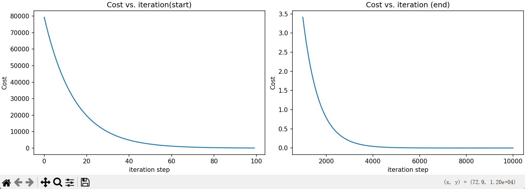
8. 可视化成本与迭代过程

# 成本随迭代变化（前后两段）
fig, (ax1, ax2) = plt.subplots(1, 2, constrained_layout=True, figsize=(12,4))
ax1.plot(J_hist[:100])
ax2.plot(1000 + np.arange(len(J_hist[1000:])), J_hist[1000:])
ax1.set_title("Cost vs. iteration(start)"); ax2.set_title("Cost vs. iteration (end)")
ax1.set_ylabel('Cost')     ; ax2.set_ylabel('Cost')
ax1.set_xlabel('iteration step')  ; ax2.set_xlabel('iteration step')
plt.show()

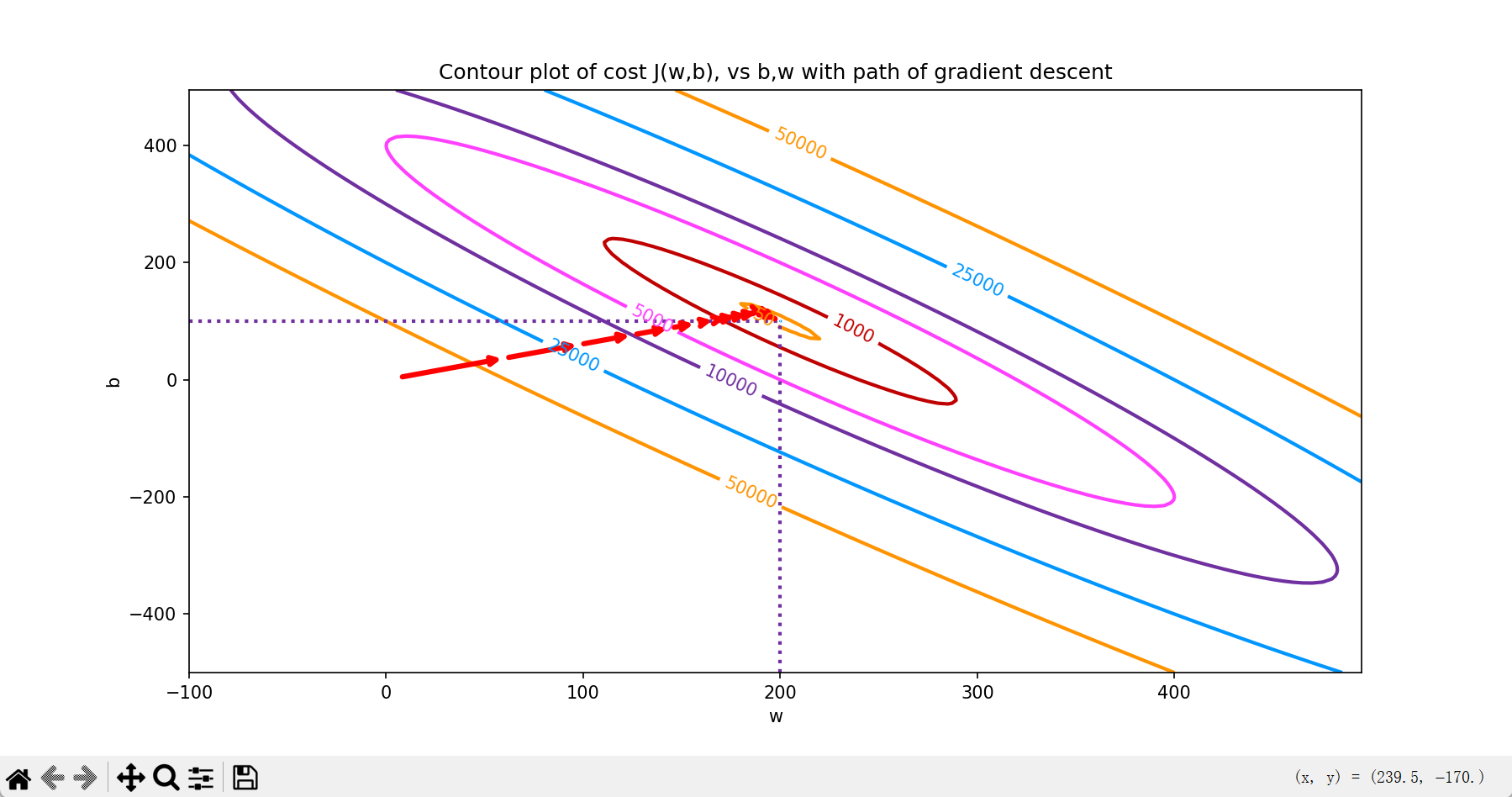
# 等高线图看梯度下降路径
fig, ax = plt.subplots(1,1, figsize=(12, 6))
plt_contour_wgrad(x_train, y_train, p_hist, ax)
plt.show()

效果：

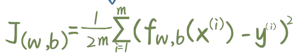
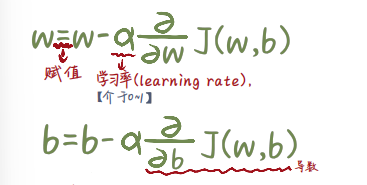
• 梯度下降的核心逻辑

  • 成本函数：
  • 梯度：

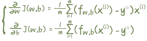
• 参数更新：

• 学习率 α 的影响

  • 太小：收敛极慢，需要很多次迭代
  • 太大：成本不下降反而上升，参数来回震荡发散