Python 二手车估价案例

在这个案例中，我们将通过数据分析和机器学习来估算二手车的价格。虽然数据集有一些缺失值和复杂性，但我们将从读取数据开始，一步一步解决问题。下面是整个过程的详细步骤。

1. 读取数据

首先，导入需要的库。这是数据科学项目的第一步：

import numpy as np
import pandas as pd
import matplotlib.pyplot as plt
import seaborn as sns
import datetime
%matplotlib inline

# 设置中文字体
plt.rcParams['font.sans-serif'] = ['KaiTi']
plt.rcParams['axes.unicode_minus'] = False

由于我们的数据文件是 TXT 格式，并且没有列名，因此在读取数据时需要手动指定列名。我们用 data 来装训练集，用 data2 来装测试集。

columns = ['carid', 'tradeTime', 'brand', 'serial', 'model', 'mileage', 
           'color', 'cityid', 'carCode', 'transferCount', 'seatings', 
           'registerDate', 'licenseDate', 'country', 'maketype', 'modelyear', 
           'displacement', 'gearbox', 'oiltype', 'newprice', 'AF1', 
           'AF2', 'AF3', 'AF4', 'AF5', 'AF6', 'AF7', 'AF8', 'AF9', 
           'AF10', 'AF11', 'AF12', 'AF13', 'AF14', 'AF15', 'price']

data = pd.read_csv('附件1：估价训练数据.txt', sep='\t', header=None, names=columns)
data2 = pd.read_csv('附件2：估价验证数据.txt', sep='\t', header=None, names=columns[:-1])

# 展示前五行
print(data.head())

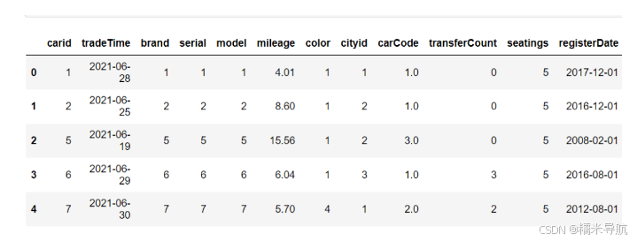
2. 数据初步检查

接下来，我们需要查看数据的基本信息和类型。

data.infer_objects()
data2.infer_objects()
data.info()
data2.info()

通过这些信息，我们可以知道每个特征的类型及非空值的个数。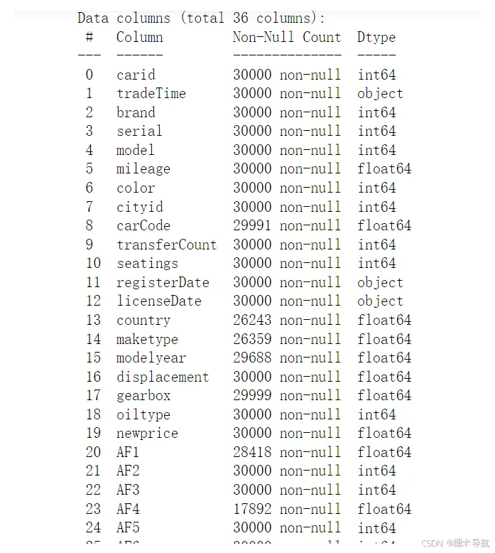

3. 数据清洗

数据清洗是至关重要的一步。首先，我们要观察缺失值的情况。

import missingno as msno

# 观察缺失值
msno.matrix(data)
msno.matrix(data2)

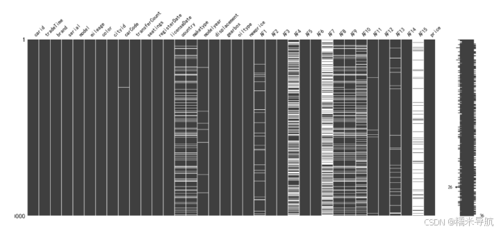
图中的黑色部分表示有数据，白色部分表示缺失数据。接下来，我们将处理这些缺失值。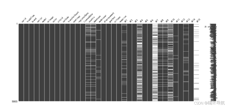

3.1 删除无用特征

• 删除 ID 列：它对模型没有帮助。

data.drop('carid', axis=1, inplace=True)
ID = data2['carid']

• 删除全为空的行：

data.dropna(how='all', inplace=True)
data2.dropna(how='all', inplace=True)

• 删除取值唯一的特征：

for col in data.columns:
    if len(data[col].value_counts()) == 1:
        data.drop(col, axis=1, inplace=True)

• 删除缺失比例过高的列：

miss_ratio = 0.15
for col in data.columns:
    if data[col].isnull().sum() > data.shape[0] * miss_ratio:
        data.drop(col, axis=1, inplace=True)

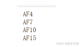
3.2 处理数值型和非数值型数据

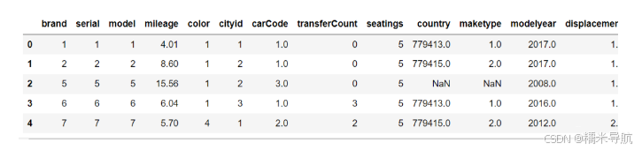
查看数值型数据：

pd.set_option('display.max_columns', 30)
data.select_dtypes(exclude=['object']).head()

对于不需要的变量，进行删除：

data.drop('AF13', axis=1, inplace=True)  # 删除不知道含义的日期变量

处理非数值型数据：

data.drop(['licenseDate', 'AF12'], axis=1, inplace=True)

3.3 填充缺失值

可以用均值、中位数、众数等方式填充缺失值：

data.fillna(data.median(), inplace=True)
data.fillna(method='ffill', inplace=True)
data2.fillna(data2.median(), inplace=True)
data2.fillna(method='ffill', inplace=True)

4. 特征工程

4.1 处理时间特征

计算车龄（以天为单位）：

data['age'] = (pd.to_datetime(data['tradeTime']) - pd.to_datetime(data['registerDate'])).map(lambda x: x.days)
data2['age'] = (pd.to_datetime(data2['tradeTime']) - pd.to_datetime(data2['registerDate'])).map(lambda x: x.days)

data.drop(['tradeTime', 'registerDate'], axis=1, inplace=True)
data2.drop(['tradeTime', 'registerDate'], axis=1, inplace=True)

4.2 独热编码

对分类变量进行独热编码：

data = pd.get_dummies(data)
data2 = pd.get_dummies(data2)

# 对于独热编码后特征数量不一致的情况处理
for col in data.columns:
    if col not in data2.columns:
        data2[col] = 0

5. 数据可视化探索

5.1 特征变量的箱线图

plt.figure(figsize=(20, 8))
plt.boxplot(x=data.values, labels=data.columns)
plt.show()

5.2 核密度图对比

plt.figure(figsize=(20, 8))
for col in data.columns:
    sns.kdeplot(data[col], color="Red", shade=True)
    sns.kdeplot(data2[col], color="Blue", shade=True)
    plt.title(f'{col} 核密度图')
    plt.xlabel(col)
    plt.show()

6. 模型选择和训练

我们将使用多种回归算法进行比较：

from sklearn.model_selection import train_test_split

X_train, X_val, y_train, y_val = train_test_split(data, data['price'], test_size=0.2, random_state=0)

训练不同的模型并比较其性能：

from sklearn.linear_model import LinearRegression
from sklearn.ensemble import RandomForestRegressor
from sklearn.ensemble import GradientBoostingRegressor
from xgboost import XGBRegressor
from lightgbm import LGBMRegressor

models = {
    "Linear Regression": LinearRegression(),
    "Random Forest": RandomForestRegressor(n_estimators=100),
    "Gradient Boosting": GradientBoostingRegressor(),
    "XGBoost": XGBRegressor(),
    "LightGBM": LGBMRegressor()
}

for name, model in models.items():
    model.fit(X_train, y_train)
    score = model.score(X_val, y_val)
    print(f'{name} 验证集准确率: {score:.4f}')

7. 超参数调优

我们将使用网格搜索和随机搜索来优化模型的超参数。

7.1 随机搜索

from sklearn.model_selection import RandomizedSearchCV

param_distributions = {
    'max_depth': range(4, 10),
    'subsample': np.linspace(0.5, 1, 5),
    'num_leaves': [15, 31, 63, 127],
    'colsample_bytree': [0.6, 0.7, 0.8, 1.0]
}

model = RandomizedSearchCV(estimator=LGBMRegressor(random_state=0), param_distributions=param_distributions, n_iter=200)
model.fit(X_train, y_train)
print(f'最优参数: {model.best_params_}')

7.2 网格搜索

from sklearn.model_selection import GridSearchCV

param_grid = {
    'learning_rate': np.linspace(0.05, 0.3, 6),
    'n_estimators': [100, 500, 1000, 1500, 2000]
}

model = GridSearchCV(estimator=LGBMRegressor(random_state=0), param_grid=param_grid, cv=3)
model.fit(X_train, y_train)
print(f'最优参数: {model.best_params_}')

8. 结果预测与保存

最后，我们使用模型对测试集进行预测，并将结果保存到 CSV 文件中。

pred = model.predict(data2)
df = pd.DataFrame(ID)
df['price'] = pred
df.to_csv('二手车估价预测结果.csv', index=False)

总结

通过这一步一步的流程，我们完成了二手车价格的估算。虽然数据清洗和特征工程的过程可能有点复杂，但这是确保模型准确性的重要步骤。在未来的实际应用中，可以根据具体的数据情况调整处理方法和模型选择。希望这个案例能帮助你更好地理解数据预处理和模型训练的过程！