性能可视化监控:grafana、influxdb、netdata
官方文档:https://grafana.com/docs/grafana/latest/
github 地址:https://github.com/grafana/grafana
性能监控 netdata / prometheus / grafana:https://zhuanlan.zhihu.com/p/604041531
netdata (开源分布式实时监控系统) 官网:https://www.netdata.cloud/
influxdb(开源时间序列数据库):https://github.com/influxdata/influxdb
1、Grafana 简介
Grafana 是一个开源的度量分析与可视化套件。经常被用作基础设施的时间序列数据和应用程序分析的可视化,它在其他领域也被广泛的使用包括工业传感器、家庭自动化、天气和过程控制等。
Grafana 支持许多不同的数据源。每个数据源都有一个特定的查询编辑器,该编辑器定制的特性和功能是公开的特定数据来源。
Grafana 的监控是基于数据库的,通过插件获取到服务器性能并存储到数据库中,然后使用Grafana 连接数据库形成可视化的图表。
官方支持以下数据源:Graphite,InfluxDB,OpenTSDB,Prometheus,Elasticsearch,CloudWatch和KairosDB。每个数据源的查询语言和能力都是不同的。你可以把来自多个数据源的数据组合到一个仪表板,但每一个面板被绑定到一个特定的数据源,它就属于一个特定的组织。
Grafana 特性
官方在线的 demo,可以体验 Grafana 最新特性 :http://play.grafana.org/
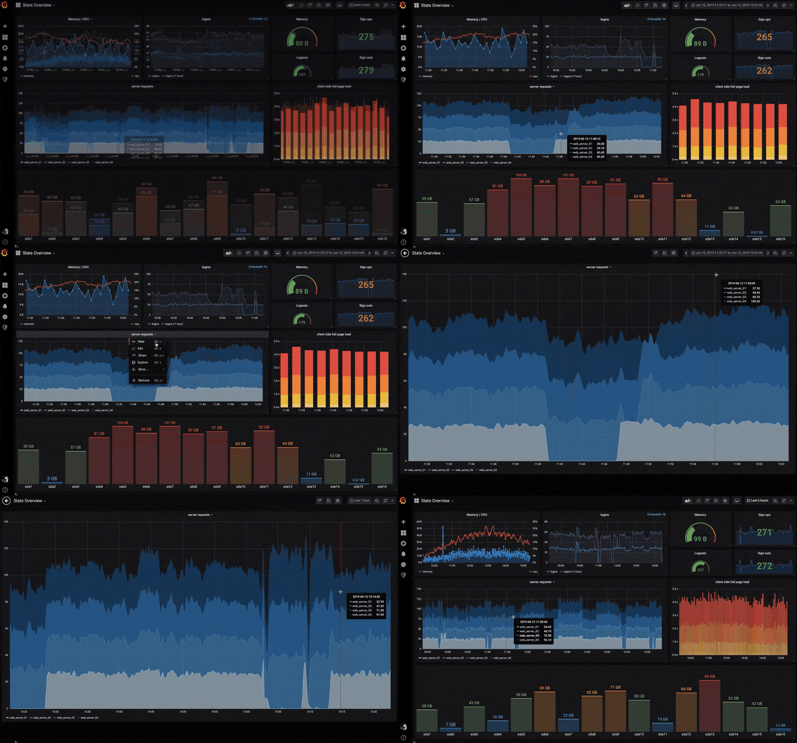
可视化
快速灵活的可视化以及多种选择,使你可以以任何方式可视化数据。官方库中具有丰富的仪表盘插件,比如热图、折线图、图表等多种展示方式。
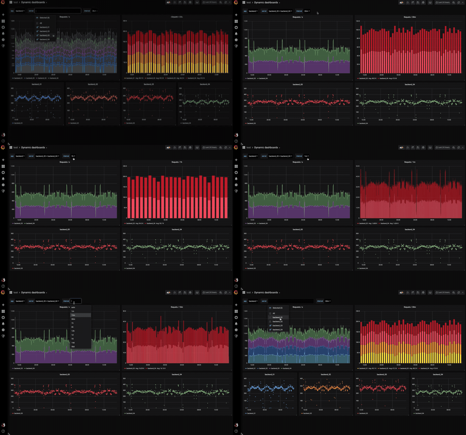
动态仪表盘
使用模板变量创建动态且可重复使用的仪表板,这些模板变量显示在仪表板顶部。
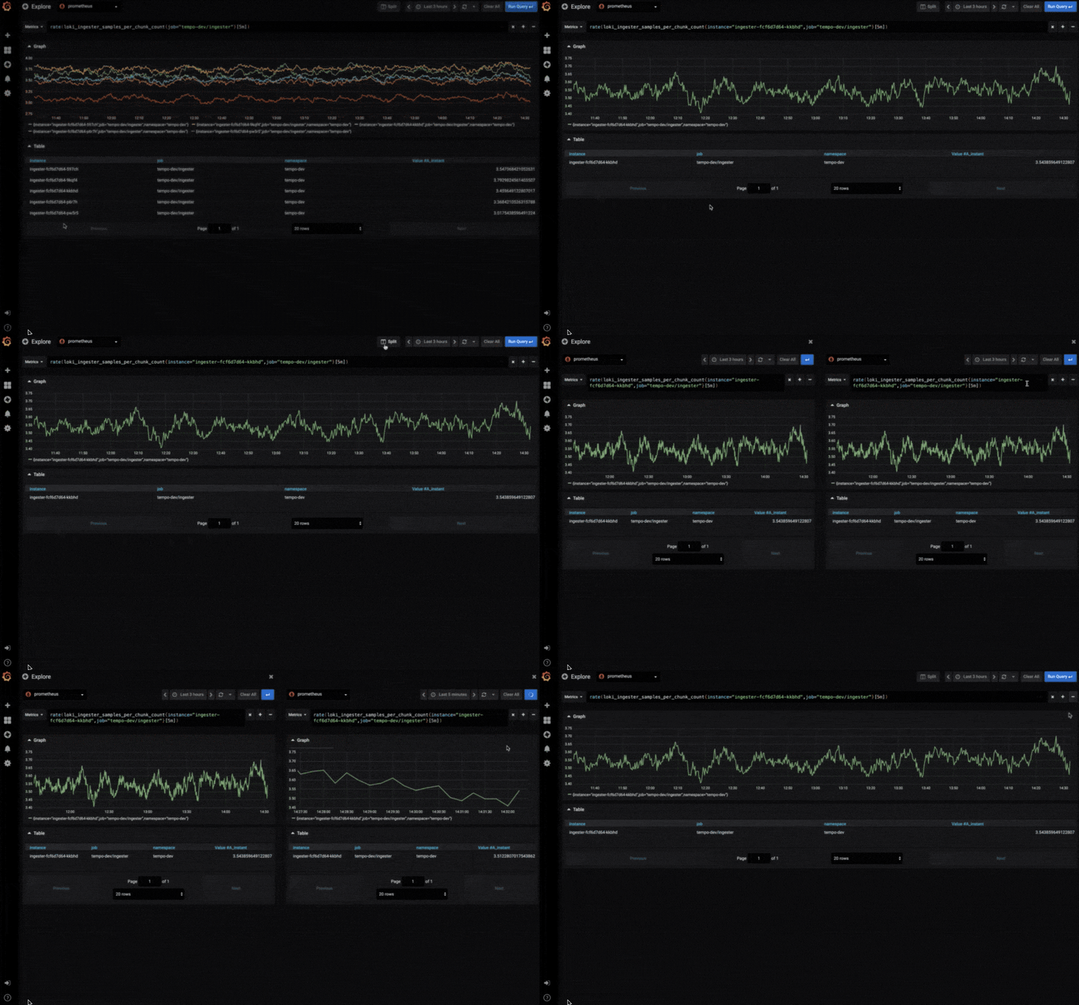
探索指标
通过临时查询和动态明细浏览数据。拆分视图并排比较不同的时间范围,查询和数据源。
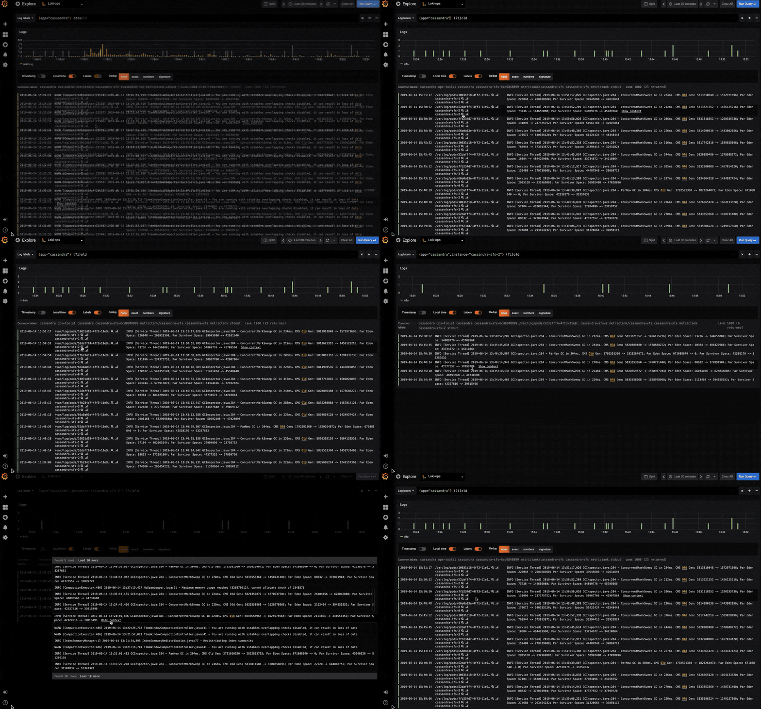
探索日志
快速搜索所有日志或实时流式传输(与 Loki 数据源配合使用效果最佳)。
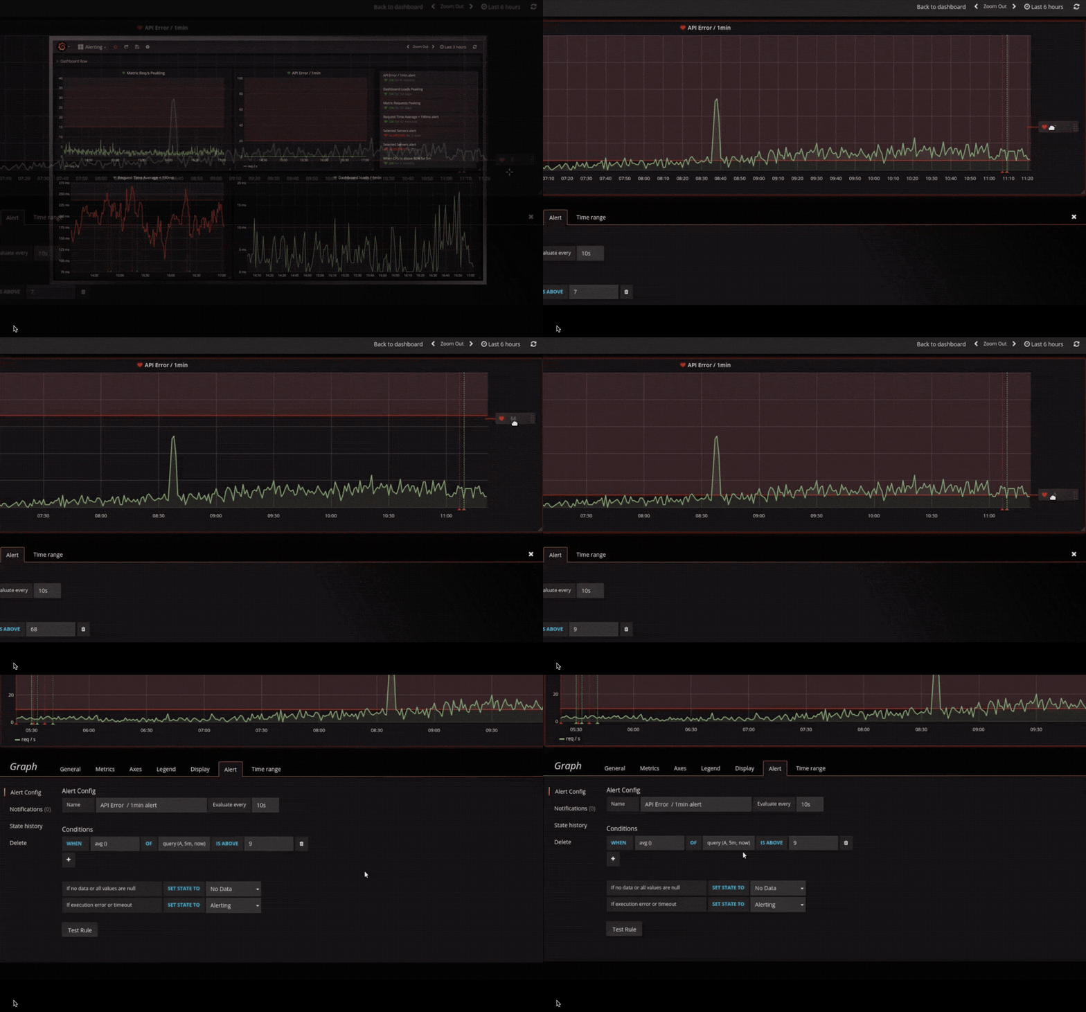
警报
以可视方式定义最重要指标的警报规则。Grafana 将不断评估并向 Slack,PagerDuty,VictorOps 和 OpsGenie 等系统发送通知。
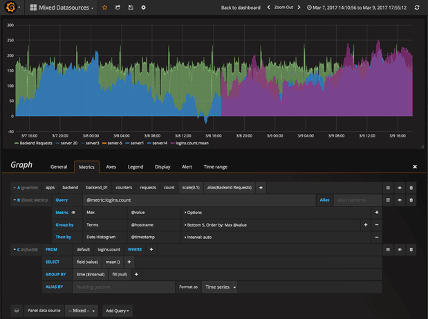
混合数据源
在同一张图中混合使用不同的数据源!你可以为每个查询指定数据源(适用于自定义数据源)。
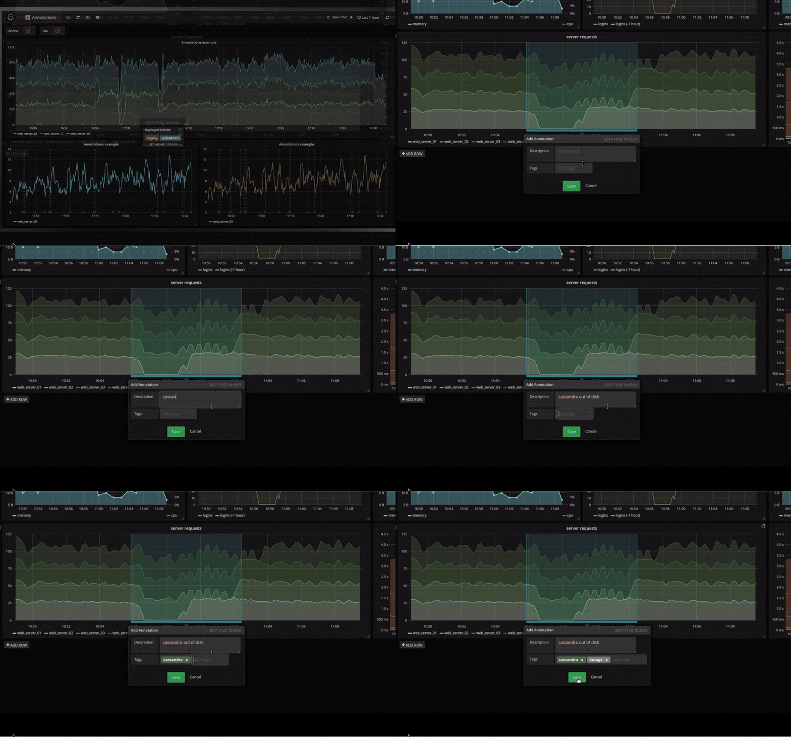
注解
使用来自不同数据源的丰富事件注释图形。将鼠标悬停在事件上会显示完整的事件元数据和标签。
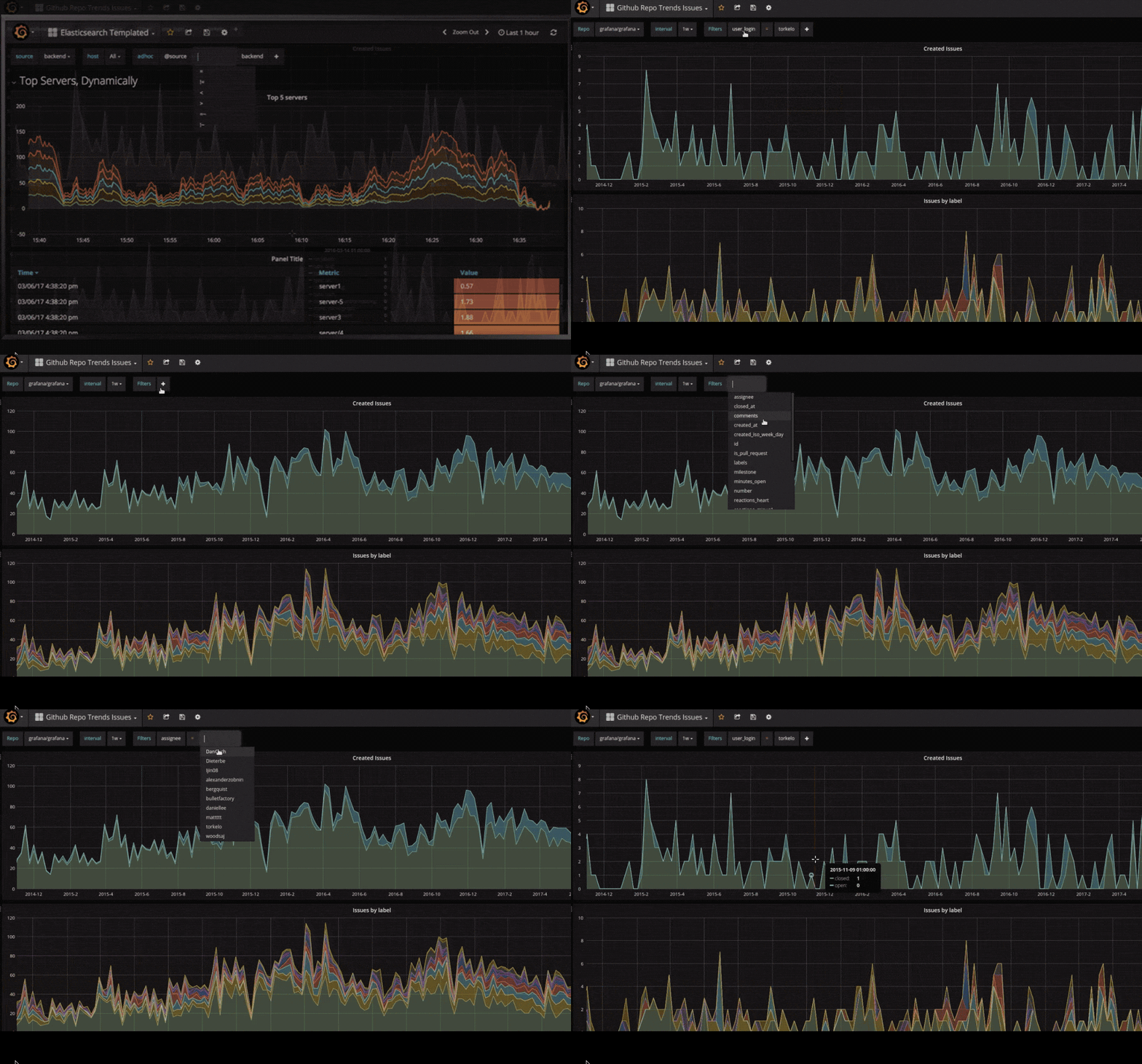
临时过滤器
临时过滤器允许您即时创建新的键/值过滤器,这些过滤器会自动应用于使用该数据源的所有查询。
在线资源
grafana 提供了一些在线资源,可以帮助使用者更方便的使用 grafana,比如在线 dashboard( https://grafana.net/dashboards ) 可以帮助快速生成一个美观的 dashboard,不用自己花心思去布局了,在线插件仓库( https://grafana.net/plugins )可以帮助连接其他数据源,如 zabbix,Open-Falcon 等,或添加其他展示图表,如饼图(Pie chat)。合理利用这些在线资源可以让 grafana 更加完善易用。
- grafana官方文档: http://docs.grafana.org/
- elasticsearch官方文档: https://www.elastic.co/guide/en/elasticsearch/reference/2.4/index.html
ELK stack 中文指南 之 Grafana:https://elkguide.elasticsearch.cn/elasticsearch/other/grafana.html
下载、安装
安装下载:https://grafana.com/grafana/download
这里以 windows 为例,下载完压缩包,直接解压,执行 grafana-server.exe
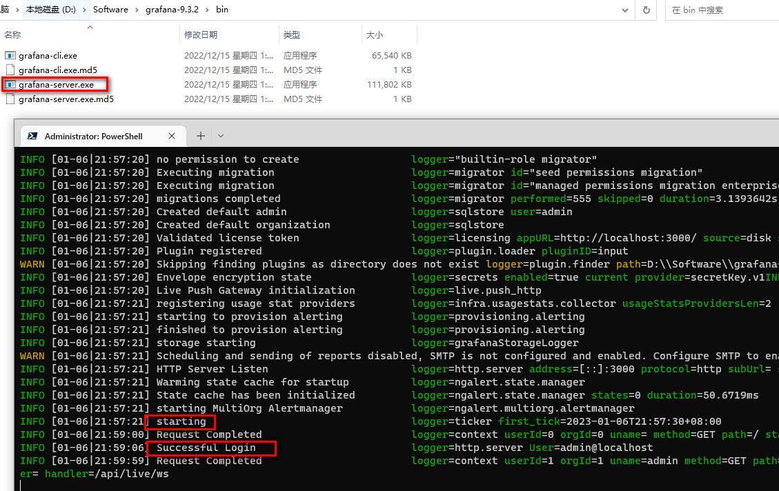
登录 grafana
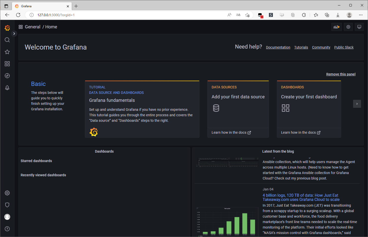
- 登录 grafana 界面:http://127.0.0.1:3000
- 默认用户和密码均为:admin
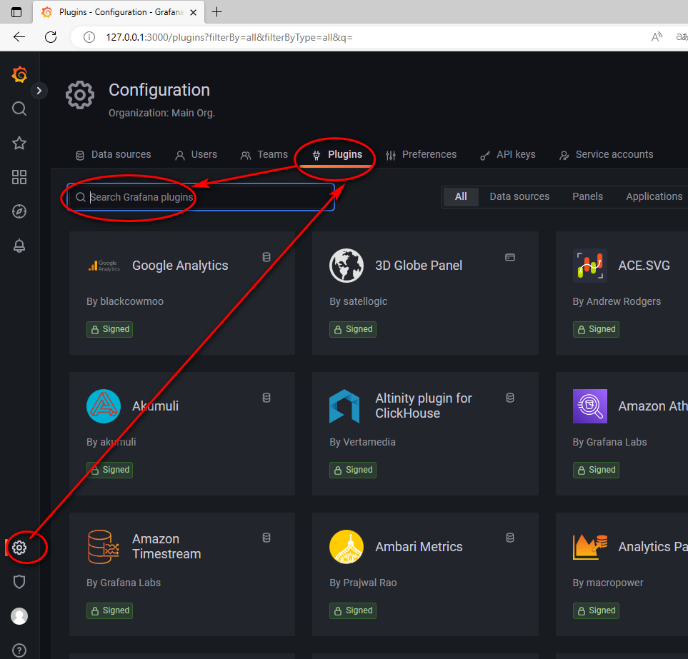
Grafana 安装 插件
这里搜索 zabbix、clock 插件并安装
插件安装完成后位置:D:\Software\grafana-9.3.2\data\plugins
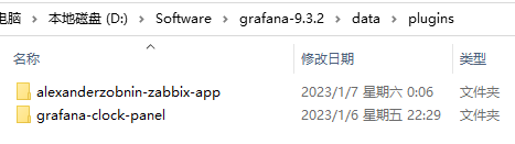
注意:安装完插件后,需要重启 grafana-server,插件才能生效。。。
clock 插件安装之后直接可以使用,无需设置。
zabbix 需要设置添加数据源:https://blog.csdn.net/weixin_62352862/article/details/128254050
2、Grafana 的 Dashboards(看板、仪表盘)
创建 Dashboards
Prometheus入门教程(三):Grafana 图表配置快速入门:https://mp.weixin.qq.com/s/sA0nYevO8yz6QLRz03qJSw
Dashboard(仪表盘)与 Panel(面板)是 Prometheus 的基本单元,所有的监控数据都会通过这两个东西来呈现。Panel 是 Prometheus 中数据呈现的最小单元。
一个 Dashboard 中可以有多个 Panel。我们看到的 Dashboard 数据,都是由一个个 Panel 构成的。Panel 的设置区域一共可以分为三部分:
- 预览区:用来预览设置的图表。
- 数据设置区:用来设置数据源、数据指标等。
- 图表设置区:用来对图表的名称等进行设置。
Dashboard 就是一个大的面板,里面包含了无数个图表(Panel)
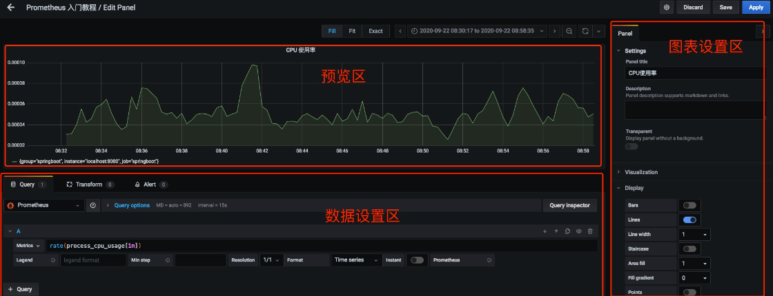
数据设置区可以分为三个设置区域,分别是:
- 查询设置区:设置查询数据的数据源、指标等。
- 转换设置区:可以对查询出来的数据进行过滤等。
- 告警设置区:可以对设置的指标设置告警规则。
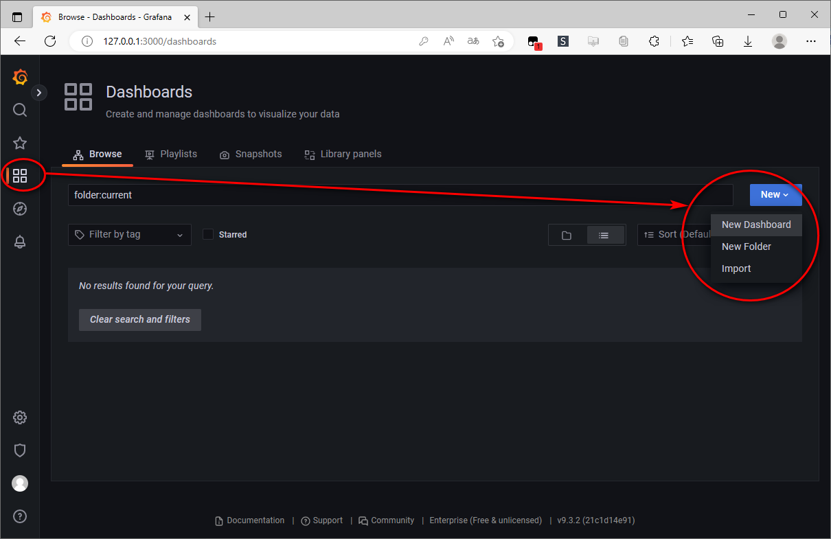
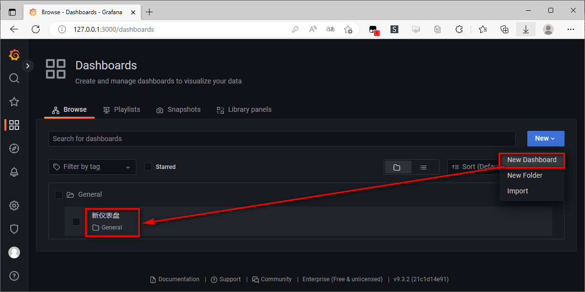
手动 创建 Dashboards
可以根据自己的需求手动新建一个 Dashboard。除此之外,https://grafana.com/grafana/dashboards 上还有很多公共的 Dashboard 可以选用。
导入 公共 Dashboards
更多的模板,我们也可以去 grafana 官网下载监控面板
下载网址:https://grafana.com/grafana/dashboards?dataSource=prometheus
仪表盘 添加 面板(panel)
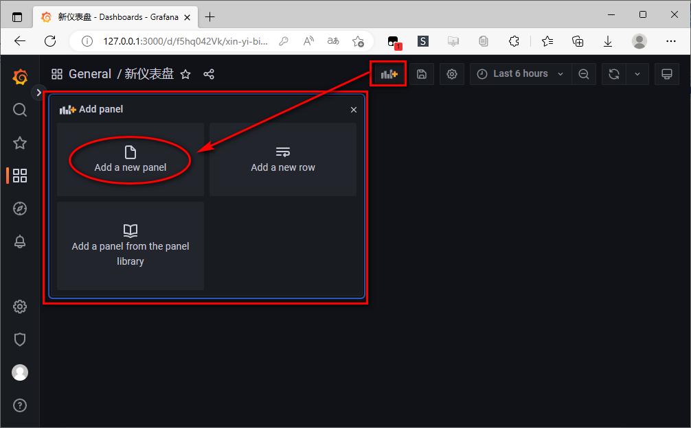
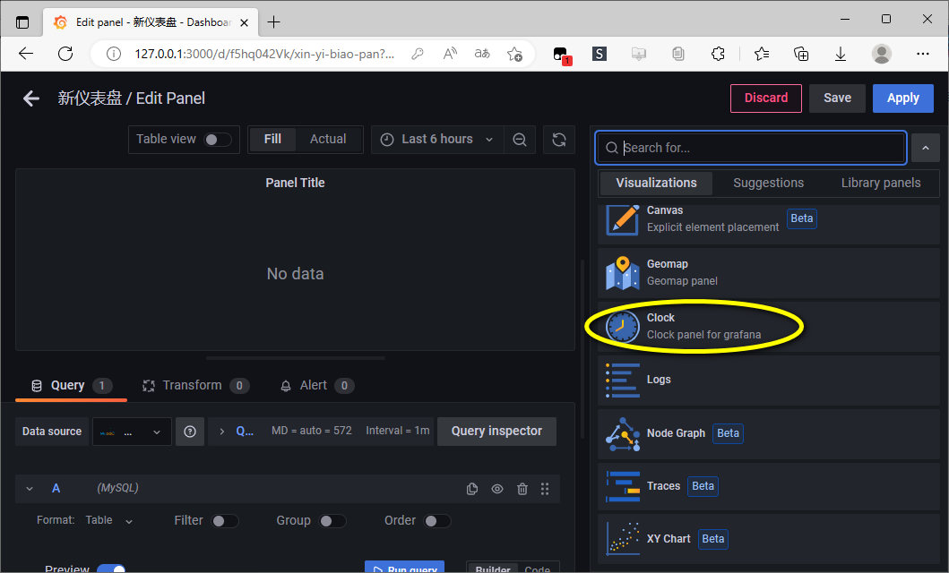
面板(panel) 的 可视化
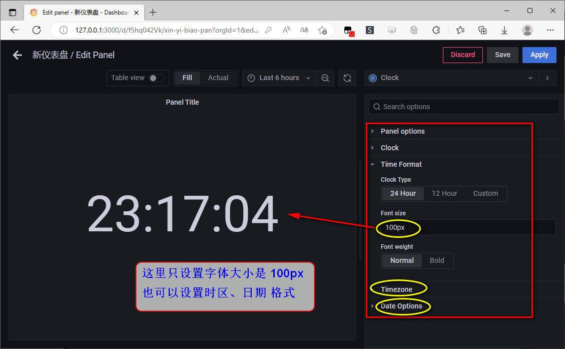
设置 面板的可视化为 clock
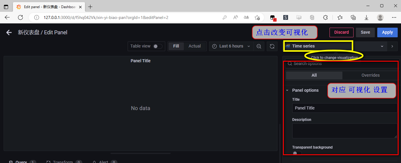
示例:面板可视化 --- 添加 时间 仪表板
仪表盘 布局
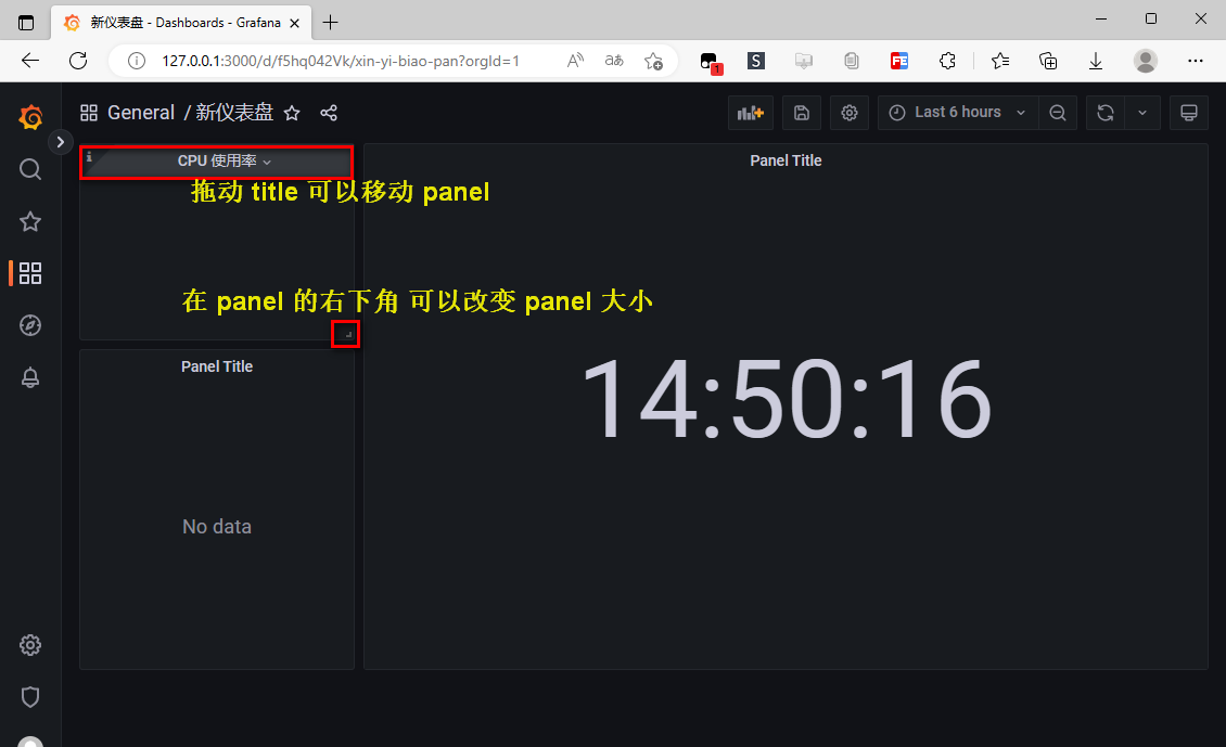
示例:面板可视化 --- 创建 CPU、内存使用率 仪表板
关键字:grafana cpu
Prometheus + Grafana 监控系统部署:https://zhuanlan.zhihu.com/p/425304902
主机基础监控(cpu,内存,磁盘,网络):https://grafana.com/grafana/dashboards/9276-1-cpu/
clock、zabbix 简单使用:https://www.zhangshengrong.com/p/v710KdGrXM/
示例:微服务监控 - Grafana 使用教程
:https://makeoptim.com/service-mesh/prometheus-grafana
3、Grafana 使用教程
:https://blog.csdn.net/bbwangj/article/details/81109615
1、登录grafana 界面
2、配置Grafana启用zabbix插件
3、配置Zabbix数据源
4、添加仪表板(仪表盘的使用)、面板
5、创建流量监控图形
6、仪表盘模板功能
7、查询格式
8、变量的使用
4、爬虫可视化动态监控
grafana + influxdb + MongoDB
爬虫可视化动态监控:https://www.jianshu.com/p/9de223e05a5e
原理:爬虫将抓取的数据写入MongoDB,InfluxDB从MongoDB获取数据抓取情况,Grafana 从 InfluxDB 中获取爬虫抓取数据情况并做图形化展示。
grafana + influxdb
scrapy、scrapy-redis 使用 grafana、influxdb 可视化监控
架构说明
- Scrapy:替换内置
STATS_CLASS,爬虫运行指标定时推送到 InfluxDB 2.x(时序库)PyPI - scrapy‑redis:分布式爬虫;Redis‑exporter 采集 Redis 队列深度(待爬 URL 队列长度)
- Grafana:对接 InfluxDB 数据源,做大盘可视化、告警
Scrapy 项目接入 InfluxDB(scrapy‑influxdb‑exporter),该库替换 Scrapy 内置统计收集器,自动把爬虫全部 stats 写入 InfluxDB2,兼容 scrapy‑redis 分布式爬虫
安装依赖:pip install scrapy-influxdb-exporter influxdb-client
修改 settings.py
# ========= InfluxDB2 监控配置 =========
INFLUXDB_HOST = "http://127.0.0.1:8086"
INFLUXDB_ORG = "crawler-org"
INFLUXDB_BUCKET = "scrapy-stats"
INFLUXDB_TOKEN = "my‑super‑secret‑token"
INFLUXDB_MEASUREMENT_NAME = "scrapy_stats"

# 核心:替换Scrapy内置统计类,所有stats自动上报InfluxDB
STATS_CLASS = "scrapy_influxdb_exporter.statscollectors.InfluxDBStatsCollector"

# 上报间隔,单位秒,不要太小,建议10‑30s
STATS_INTERVAL = 15
上报指标自动包含:
response_received_count、item_scraped_count、item_dropped_countlog_count/ERROR、downloader/request_count、downloader/response_status_count/403/429/500- scrapy‑redis 关键指标:
scheduler/enqueued/redis、scheduler/dequeued/redis(redis 出入队列计数)
scrapy‑Redis 额外监控:Redis 待爬队列深度。crapy‑redis 队列长度(待爬 url 数量)不会自动上报,必须单独采集,是分布式爬虫最重要指标。
方式 A:写简单脚本定时写入 InfluxDB。后台运行脚本就可以采集每个爬虫 redis 待爬队列长度。
# redis_queue_monitor.py
import time
import redis
from influxdb_client import InfluxDBClient, Point

r = redis.Redis(host="127.0.0.1", port=6379, decode_responses=False)
client = InfluxDBClient(url="http://127.0.0.1:8086", token="my‑super‑secret‑token", org="crawler‑org")
write_api = client.write_api()

# 你的spider名字列表
spiders = ["spider_a","spider_b"]

while True:
    for name in spiders:
        key = f"{name}:requests"
        queue_len = r.llen(key)
        p = Point("scrapy_redis_queue").tag("spider",name).field("queue_length", queue_len)
        write_api.write(bucket="scrapy‑stats", org="crawler‑org", record=p)
    time.sleep(15)
方式 B:Prometheus + redis‑exporter
- scrapy‑prometheus‑exporter:Scrapy 暴露 Prometheus metrics HTTP 接口
- redis‑exporter:采集 scrapy‑redis Redis 队列指标(待爬任务数)
- prometheus:拉取指标、存储时序数据。对比 InfluxDB:Prometheus 是云原生标准,生态成熟,告警能力强,更适合爬虫生产监控。
- grafana:可视化大盘、告警
Grafana 配置 InfluxDB 数据源
- Grafana → Connections → Data sources → Add data source → 选择 InfluxDB
- Query language 选择 Flux(InfluxDB2 必须 Flux,不要选 InfluxQL)
- URL:
http://influxdb2:8086 - Token:填入
my‑super‑secret‑token - Organization:
crawler‑org - Bucket:
scrapy‑stats保存并测试。
常用 Flux 查询语句(直接复制到 Grafana 面板)
每秒抓取 Item 速率
from(bucket:"scrapy-stats")
  |> range(start: v.timeRangeStart, stop:v.timeRangeStop)
  |> filter(fn: (r) => r._measurement == "scrapy_stats" and r._field == "item_scraped_count")
  |> aggregateWindow(every: 10s, fn: difference)
HTTP 403/429/500 错误数量
from(bucket:"scrapy-stats")
  |> range(start: v.timeRangeStart)
  |> filter(fn: (r) => r._measurement == "scrapy_stats" and r._field =~ /downloader\/response_status_count\/403|429|500/)
  |> aggregateWindow(every:10s, fn:difference)
scrapy‑redis 待爬队列长度
from(bucket:"scrapy-stats")
  |> range(start: v.timeRangeStart)
  |> filter(fn: (r) => r._measurement == "scrapy_redis_queue" and r._field == "queue_length")
ERROR 日志计数
from(bucket:"scrapy-stats")
  |> range(start: v.timeRangeStart)
  |> filter(fn: (r) => r._measurement == "scrapy_stats" and r._field == "log_count/ERROR")
  |> aggregateWindow(every: 10s, fn: difference)
大盘面板建议
- 数字面板:总抓取 Item、当前待爬队列长度
- 折线图:Item 抓取速率、QPS
- 折线图:403/429/500 错误趋势
- 折线图:Redis 待爬队列深度
- 告警:队列长时间不变(爬虫卡死);错误率超过阈值触发告警
Netdata
官网有在线演示 demo
5、python 进行数据可视化
现在市面上可以使用 python 的可视化库多如牛毛,各有各的优点。一个经典的可视化库 matplotlib 它是基于 NumPy 的一个数据可视化工具,内置了非常多图给我们使用。下载这个库
python -m pip install matplotlib
示例:画 sin 和 cos线
import numpy as np
import matplotlib.pyplot as plt

x = np.linspace(-np.pi, np.pi, 256)

cos = np.cos(x)
sin = np.sin(x)

plt.plot(x, cos, '--', linewidth=2)
plt.plot(x, sin)

plt.show()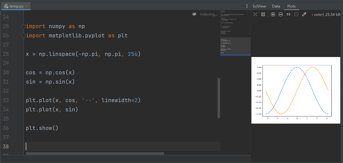
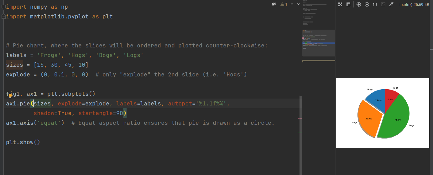
画个饼图
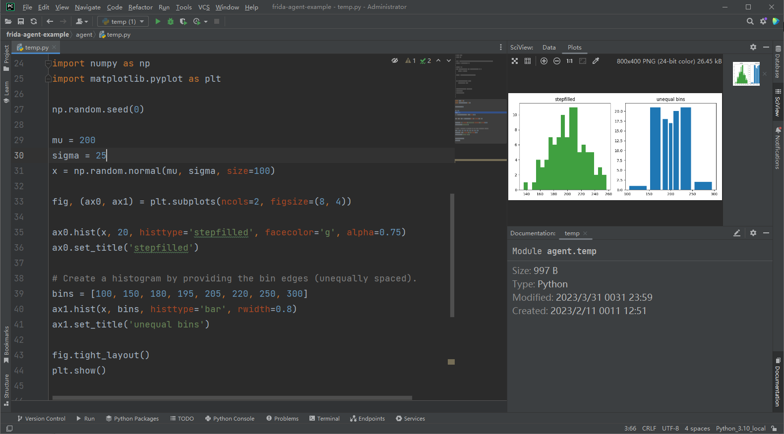
画直方图
更多关于 matplotlib 的文档可以到以下链接查看:https://matplotlib.org/2.0.2/contents.html
seaborn
seaborn 是基于 matplotlib 的库,所以有更加高级的接口给我们使用,相对来说更加简单使用一些
画个散点图。安装:pip install seaborn
数据源:https://github.com/mwaskom/seaborn-data
下载 seaborn-data,然后解压后,将文件拖进电脑中 seaborn-data 的空文件夹里即可。
import numpy as np
import pandas as pd
import matplotlib.pyplot as plt
import seaborn as sns

sns.set(style="darkgrid")

tips = sns.load_dataset("tips")
sns.relplot(x="total_bill", y="tip", data=tips)
plt.show()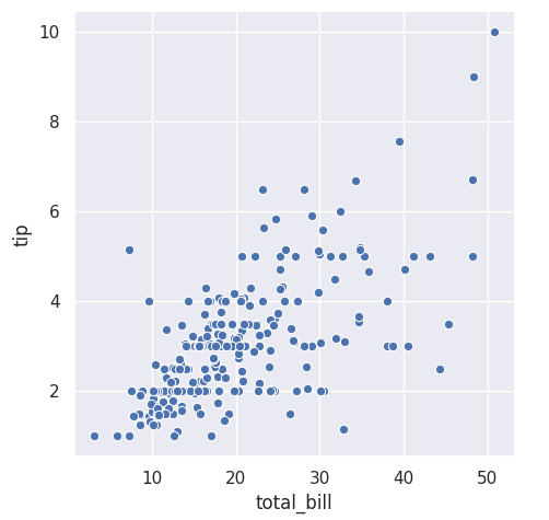
画个折线图
fmri = sns.load_dataset("fmri")
sns.relplot(x="timepoint", y="signal", hue="event", kind="line", data=fmri);
plt.show()
画个直方图
titanic = sns.load_dataset("titanic")
sns.catplot(x="sex", y="survived", hue="class", kind="bar", data=titanic);
plt.show()
更多关于 seaborn:https://seaborn.pydata.org/index.html
百度开源的数据可视化的 echarts 的库
来画个直方图
from pyecharts.charts import Bar
from pyecharts import options as opts

bar = (
    Bar()
    .add_xaxis(["衬衫", "毛衣", "领带", "裤子", "风衣", "高跟鞋", "袜子"])
    .add_yaxis("商家A", [114, 55, 27, 101, 125, 27, 105])
    .add_yaxis("商家B", [57, 134, 137, 129, 145, 60, 49])
    .set_global_opts(title_opts=opts.TitleOpts(title="某商场销售情况"))
)
bar.render()
画个饼图
def pie_base() -> Pie:
    c = (
        Pie()
        .add("", [list(z) for z in zip(Faker.choose(), Faker.values())])
        .set_global_opts(title_opts=opts.TitleOpts(title="Pie-基本示例"))
        .set_series_opts(label_opts=opts.LabelOpts(formatter="{b}: {c}"))
    )
    return c

# 需要安装 snapshot_selenium
make_snapshot(driver, pie_base().render(), "pie.png")
再来画个词云图
words = [
    ("Sam S Club", 10000),
    ("Macys", 6181),
    ("Amy Schumer", 4386),
    ("Jurassic World", 4055),
    ("Charter Communications", 2467),
    ("Chick Fil A", 2244),
    ("Planet Fitness", 1868),
    ("Pitch Perfect", 1484),
    ("Express", 1112),
    ("Home", 865),
    ("Johnny Depp", 847),
    ("Lena Dunham", 582),
    ("Lewis Hamilton", 555),
    ("KXAN", 550),
    ("Mary Ellen Mark", 462),
    ("Farrah Abraham", 366),
    ("Rita Ora", 360),
    ("Serena Williams", 282),
    ("NCAA baseball tournament", 273),
    ("Point Break", 265),
]


def wordcloud_base() -> WordCloud:
    c = (
        WordCloud()
        .add("", words, word_size_range=[20, 100])
        .set_global_opts(title_opts=opts.TitleOpts(title="WordCloud-基本示例"))
    )
    return c

# 需要安装 snapshot_selenium
make_snapshot(driver, wordcloud_base().render(), "WordCloud.png")
更多关于 pyecharts:https://pyecharts.org

DAMO开发者矩阵,由阿里巴巴达摩院和中国互联网协会联合发起,致力于探讨最前沿的技术趋势与应用成果,搭建高质量的交流与分享平台,推动技术创新与产业应用链接,围绕“人工智能与新型计算”构建开放共享的开发者生态。
更多推荐

 7
7 0
0- 0


 已为社区贡献3条内容

所有评论(0)