稀疏高斯过程_稀疏和变分高斯过程数据量大时该怎么办_java_weixin

稀疏高斯过程

Big data is the cure for many machine learning problems. But one person’s cure can be another’s poison. Big data causes many Bayesian methods to be unpractically expensive. We need to do something or Bayesian methods are left behind the big data revolution.

大数据是解决许多机器学习问题的方法。但是一个人的治愈可能是另一个人的毒药。大数据导致许多贝叶斯方法不切实际地昂贵。我们需要做些事情，否则贝叶斯方法将被甩在大数据革命的后面。

In this article, I will explain why big data makes a very popular Bayesian machine learning method — Gaussian Process —unaffordably expensive. Then I will present Bayesian’s solution — the Sparse and Variational Gaussian Process model (SVGP model), that brings Gaussian Process back in the game.

在本文中，我将解释为什么大数据使非常流行的贝叶斯机器学习方法(高斯过程)价格昂贵。然后，我将介绍贝叶斯解决方案-稀疏和变分高斯过程模型(SVGP模型)，它将高斯过程带回游戏中。

一些符号 (Some notations)

Medium supports Unicode in text. This allows me to write many math subscript notations such as X₁ and Xₙ. But I could not write down some other subscripts. For example:

中号支持文本中的Unicode。这使我可以编写许多数学下标符号，例如X₁和Xₙ。 但是我无法写下其他一些下标。例如：

So in the text, I will use an underscore “_” to lead such subscripts, such as X_* and X_*1.

因此，在本文中，我将使用下划线“ _”引导此类下标，例如X_ *和X_ * 1 。

If some math notations render as question marks on your phone, please try to read this article from a computer. This is a known issue with some Unicode rendering.

如果某些数学符号在您的手机上显示为问号，请尝试从计算机上阅读本文。这是某些Unicode渲染的已知问题。

高斯过程回归模型 (The Gaussian Process regression model)

Suppose we have some training data (X, Y). Both X and Y are float vectors of length n. So n is the number of training data points. We want to find a regression function from X to Y. This is a typical regression task. We can use the Gaussian Process regression model (GPR) to find such a function.

假设我们有一些训练数据(X，Y)。 X和Y均为长度为n的浮点向量。所以n是训练数据点的数量。我们想要找到从X到Y的回归函数。这是典型的回归任务。我们可以使用高斯过程回归模型(GPR)查找此类函数。

The Gaussian Process regression model is the simplest Gaussian Process model. If you need to refresh your memory, the article Understanding Gaussian Process, The Socratic Way is a great read. This model has two parts — the prior and the likelihood:

高斯过程回归模型是最简单的高斯过程模型。如果您需要刷新内存，那么这篇文章《理解高斯过程，苏格拉底式的方式》是一本不错的文章。该模型有两个部分-先验和可能性：

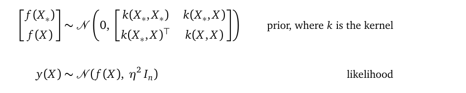
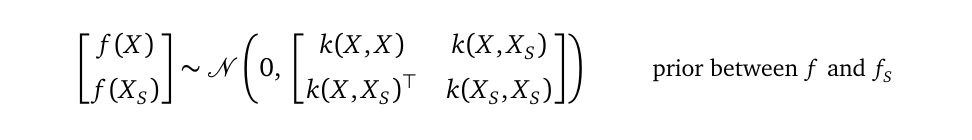
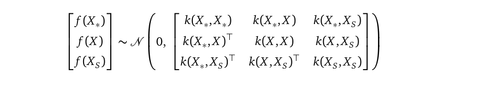
The GP priorThe Gaussian Process prior (GP prior) is a multivariate Gaussian distribution over random variable vectors f(X) and f(X_*):

GP先验高斯过程先验(GP先验)是随机变量向量f(X)和f(X_ *)上的多元高斯分布：

f(X) is a random variable vector of length n; it represents possible values of the underlying regression function at training locations X.

f(X)是长度为n的随机变量矢量；它表示潜在的回归函数在训练位置X的可能值。
f(X_*) is also a random variable vector. It represents possible values of the underlying regression function at testing locations X_*. Its length n_* depends on how many testing locations you will ask the model to make predictions for. n_* can be very large.

f(X_ *)也是一个随机变量向量。它表示在测试位置X_ *的基础回归函数的可能值。它的长度n_ *取决于您将要求模型进行预测的测试位置数。 n_ *可能非常大。

I will shorten the prior as:

我将先验缩短为：

This multivariate Gaussian distribution has zero mean, and it uses a kernel function k to define its covariance matrix. The covariance matrix k(X, X) is an n×n matrix. You have many choices over the function k, in this article, we use the squared exponential function for k:

此多元高斯分布的均值为零，并且使用核函数k定义其协方差矩阵。协方差矩阵k(X，X)是n×n矩阵。您可以对函数k进行多种选择，在本文中，我们对k使用平方指数函数：

where the signal variance σ² and lengthscale l are model parameters.

其中信号方差σ²和长度标度l是模型参数。

The likelihoodIn the likelihood, y(X) is a random variable vector of length n. It comes from a multivariate Gaussian distribution with mean f(X), and covariance η²Iₙ, where η² is a scalar model parameter called noise variance, and Iₙ is an n×n identity matrix because we assume independent observation noise.

可能性在可能性中， y(X)是长度为n的随机变量矢量。它来自均值f(X)和协方差η²Iₙ的多元高斯分布，其中η²是称为噪声方差的标量模型参数，而Iₙ是n×n单位矩阵，因为我们假设独立的观察噪声。

Training data Y is modeled as samples of the random variable vector y(X). Since y(X) depends on f(X), we also denote the likelihood as p(y(X)|f(X)). I will use y as a shorthand for y(X), and p(y|f) as the shorthand for the likelihood.

训练数据Y被建模为随机变量向量y(X)的样本。由于y(X)取决于f(X) ，因此我们也将可能性表示为p(y(X)| f(X)) 。我将y用作y(X)的简写，并将p(y | f)用作似然的简写。

Since both f and y are multivariate Gaussian random variables, and f is the mean of y, we can rewrite y as a linear transformation from f:

由于f和y都是多元高斯随机变量，并且f是y的均值，我们可以将y重写为f的线性变换：

Then we can apply the multivariate Gaussian linear transformation rule to derive the distribution of y without mentioning the random variable f:

然后我们可以应用多元高斯线性变换规则来得出y的分布，而无需提及随机变量f ：

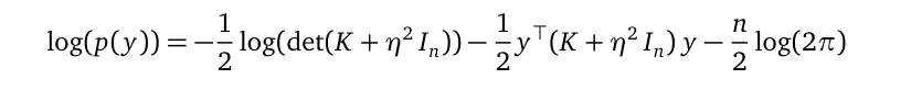
We can write down the probability density function for y:

我们可以写下y的概率密度函数：

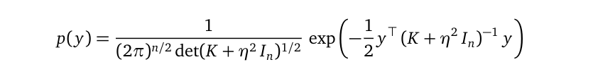
p(y) is the famous marginal likelihood.

p(y)是著名的边际似然。

Parameter learningOur Gaussian Process regression model has three model parameters, lengthscale l, signal variance σ², and observation variance η². We introduced them as part of the modeling process, but we don’t know what concrete values we should set those model parameters to. We use parameter learning to find optimal concrete values for them:

参数学习我们的高斯过程回归模型具有三个模型参数：长度尺度l ，信号方差σ²和观测方差η²。 我们在建模过程中介绍了它们，但是我们不知道应将这些模型参数设置为什么具体值。我们使用参数学习来找到最佳的具体值：

“optimal” means that with those concrete values, our model can best explain the training data (X, Y). And,

“最优”意味着，通过这些具体值，我们的模型可以最好地解释训练数据(X，Y) 。和，
“explain the training data”, in the context of probabilistic modeling (which is what we are doing), means how likely the training data is generated by our model, measured by the marginal likelihood p(y).

在概率建模(这就是我们正在做的事情)的上下文中，“解释训练数据”是指我们的模型以边际可能性p(y)衡量生成训练数据的可能性。

Once the training data X and Y are plugged in, the marginal likelihood p(y) is a function with all the model parameters l, σ², and η². To find optimal values for them, parameter learning uses gradient descent to maximize the objective function log(p(y)) with respect to those model parameters. Here is the formula for the objective function:

一旦插入了训练数据X和Y ，边际似然p(y)就是所有模型参数l，σ²和η²的函数。为了找到它们的最佳值，参数学习使用梯度下降来相对于那些模型参数最大化目标函数log(p(y)) 。这是目标函数的公式：

Making predictionsAfter we found optimal values for the model parameters (also known as calibrating the model), we are ready to make predictions. A Gaussian Process model makes predictions using the posterior distribution.

进行预测在找到模型参数的最佳值(也称为校准模型)之后，就可以进行预测了。高斯过程模型使用后验分布进行预测。

In our Gaussian Process regression model with a Gaussian likelihood, the posterior p(f_*, f|y) has a closed-form analytical expression. To make predictions for f_* at testing locations X_*, we marginalize f out from the posterior:

在具有高斯似然的高斯过程回归模型中，后验p(f_ *，f | y)具有闭合形式的解析表达式。为了对测试位置X_ *处的f_ *做出预测，我们从后验中将f边缘化：

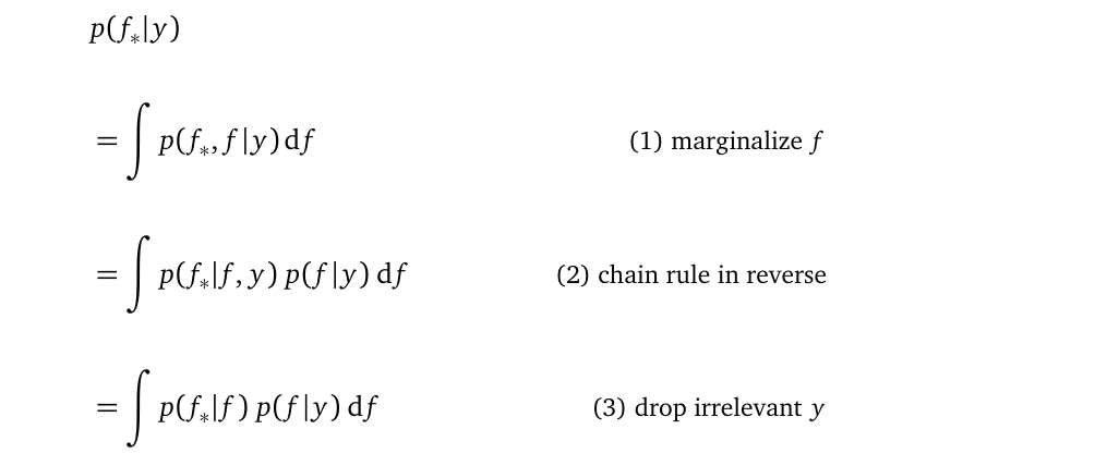
At line (3), the integrand includes two probability densities — p(f_*|f) and p(f|y). We can derive p(f_*|f) from the GP prior by applying the multivariate Gaussian conditional rule. And the Bayes rule tells us how to compute p(f|y). With its ingredients ready, we can derive the analytical expression for the predictive distribution p(f_*|y):

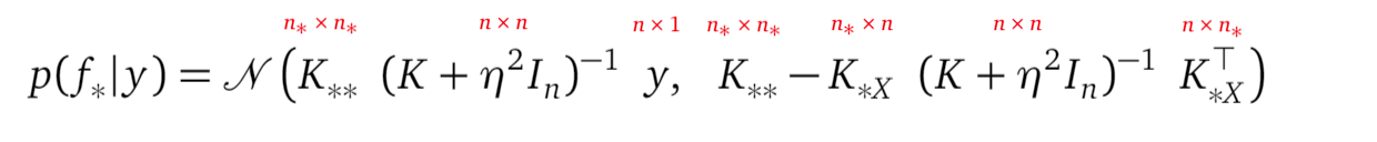
Shapes of the matrices in the above expression are shown in small red notations.

上面表达式中的矩阵形状以红色小符号表示。

Please step to Understanding Gaussian Process, the Socratic Way (the Computing the posterior section) for the full derivations of p(f_*|y).

请逐步理解高斯过程，即苏格拉底式方法 ( 计算后验部分)，以获得p(f_ * | y)的全部推导。

The predictive distribution p(f_*|y) is a distribution over the random variable vector f_*, whose length is n_*. Its structure reveals that in the Gaussian Process regression model, f_* is a linear transformation from y. The model tries to explain f_* using information from y. The kernel (the function k, the training location X, and the testing location X_*) predominantly decides the transformation from y to f_*, with the help from the observation noise η²Iₙ, of course.

预测分布p(f_ * | y)是在长度为n_ *的随机变量矢量f_ *上的分布。它的结构表明，在高斯过程回归模型中， f_ *是y的线性变换。该模型尝试使用y中的信息来解释f_ * 。当然，内核(函数k ，训练位置X和测试位置X_ * )主要决定了从y到f_ *的转换，当然还要借助观察噪声η²Iₙ 。

Please note the number of testing locations n_* can be much larger than the number of training points n. As n_* becomes larger, the matrix K_**, K_*X becomes larger, but the shape of the matrix K+η²Iₙ, which is being inverted, stays the same, n×n.

请注意，测试位置的数量n_ *可能远大于训练点的数量n 。随着n_ *变大，矩阵K _ ** ， K_ * X变大，但是矩阵K +η²Iₙ的形状被倒置，保持不变， n×n 。

矩阵求逆的诅咒 (Curse of matrix inversion)

In this Gaussian Process regression model, both the objective function for parameter learning and the predictive distribution mention the matrix inversion (K+η²Iₙ)⁻¹. Matrix inversion is computationally expensive. The number of operations (such as adding, multiplying two numbers) in an n×n matrix inversion scale with n³, with n being the number of data points.

在此高斯过程回归模型中，用于参数学习的目标函数和预测分布都提到了矩阵求逆(K +η²Iₙ)⁻¹ 。矩阵求逆在计算上是昂贵的。 n×n矩阵求逆标度中的操作数(例如加，乘两个数)为n³，其中n为数据点数。

A Gaussian Process regression model for a dataset with 10,000 data points needs 10¹² operations to invert its covariance matrix. As a comparison, our universe contains 10⁷⁸ to 10⁸² atoms. And a dataset with 10,000 points is just tiny in modern-day standards.

具有10,000个数据点的数据集的高斯过程回归模型需要10 12运算来反转其协方差矩阵。作为比较，我们的宇宙包含10⁷⁸至10⁸²原子。在现代标准中，具有10,000点的数据集很小。

(K+σ²Iₙ)⁻¹ is the reason why it is too expensive to apply our Gaussian Process regression model to even a moderate-sized dataset.

(K +σ²Iₙ)⁻¹是将我们的高斯过程回归模型应用于中等大小的数据集过于昂贵的原因。

As an example, here is a dataset with 10,000 points:

例如，这是一个具有10,000点的数据集：

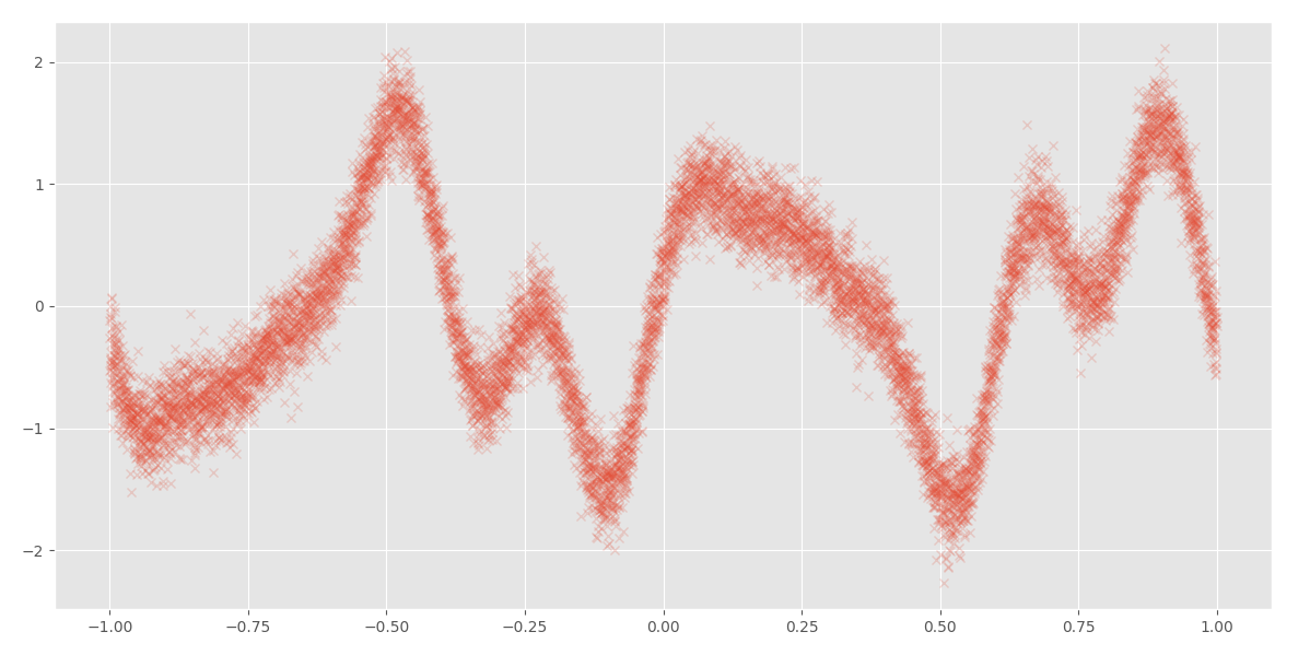
Those small red crosses are data points. When I tried to use this dataset to perform parameter learning for a Gaussian Process regression model, I saw the following warning messages and I waited for hours and then I terminated the program because I didn’t want to wait for it anymore — it is a machine learning model, not my kid, and I don’t have infinite patience for models:

那些小的红叉是数据点。当我尝试使用此数据集为高斯过程回归模型执行参数学习时，我看到以下警告消息，并且等待了几个小时，然后终止了该程序，因为我不想再等待它了-这是一个机器学习模型，不是我的孩子，而且我对模型没有无限的耐心：

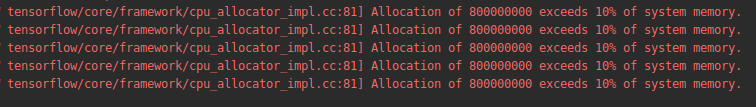
This warning message indicates that the model needs to allocate a lot of memory to perform matrix operations. And the long waiting gives you a vivid impression of the n³ scaling.

此警告消息表明模型需要分配大量内存才能执行矩阵运算。漫长的等待给您n³缩放的生动印象。

为什么会出现(K + σ²Iₙ ) ⁻¹ ？ (Why does (K+σ²Iₙ)⁻¹ appear?)

The matrix inversion (K+σ²Iₙ)⁻¹ appears in the objective function log p(y) and the predictive distribution because we are using the following factorization from the GP prior:

矩阵求逆(K +σ²Iₙ)⁻¹出现在目标函数对数p(y)和预测分布中，因为我们使用了GP之前的以下因式分解：

We use the conditional p(f_*|f) part for making predictions because this part links together what we know at training locations (namely f) and what we don’t know at testing locations (namely f_*). See the previous derivation for p(f_*|f).

我们使用条件p(f_ * | f)进行预测，因为此部分将我们在训练位置(即f )和测试点(即f_ * )所不知道的内容联系在一起。请参见p(f_ * | f)的先前推导。
We use the marginal p(f) part, combined with the likelihood p(y|f), for parameter learning because this part links together the random variables whose observations are available (namely y) and the random variables whose observations are not available (namely f). See the previous derivation for p(y).

我们将边际p(f)部分与似然性p(y | f)结合起来用于参数学习，因为该部分将其观测值可用的随机变量(即y )和其观测值不可用的随机变量(即f )。参见p(y)的先前推导。

Probability theory allows us to do the above factorization as long as:

概率理论允许我们进行上述分解，只要：

p(f_*|f) is a function that mentions both f_* and f; p(f) is a function that mentions f. This makes sure the factorization has the same API as the joint p(f_*, f).

p(f_ * | f)是同时提及f_ *和f的函数 ； p(f)是提及f的函数。这样可以确保分解与联合p(f_ *，f)具有相同的API。
both p(f_*|f) and p(f) are proper probability density functions. This makes sure that the factorization is still a valid probability density function.

p(f_ * | f)和p(f)都是适当的概率密度函数。这样可以确保分解仍然是有效的概率密度函数。

The choice of a multivariate Gaussian distribution as the prior satisfies both requirements, and it makes the derivation of p(f_*|f) and p(f) easy:

选择多元高斯分布作为先验满足这两个要求，并且使p(f_ * | f)和p(f)的推导变得容易：

derive p(f_*|f) by applying the multivariate Gaussian conditional rule on the prior.

通过在先验上应用多元高斯条件规则来推导p(f_ * | f) 。
derive p(f) by applying the multivariate Gaussian marginalization rule on the prior.

通过对先验应用多元高斯边缘化规则来推导p(f) 。

But this factorization planted the unaffordable matrix inversion because the marginal p(f) is a multivariate Gaussian distribution:

但是，由于边际p(f)是多元高斯分布，因此该分解法植入了无法承受的矩阵求逆：

and the K⁻¹ is right there in this probability density function. The marginal likelihood p(y) inherited this inversion and made its own contribution σ²Iₙ, resulting in that unaffordable term (K+σ²Iₙ)⁻¹.

在这个概率密度函数中， K⁻¹就在那里。边际似然p(y)继承了该反演并做出了自己的贡献σ²Iₙ ，从而导致了该无法承受的项(K +σ²Iₙ)⁻¹。

我们可以降采样吗？ (Can we downsample?)

Since the size of data, n, controls the shape of the covariant matrix K that we have a hard time to invert, can we select a subset of the training data? This is called downsampling. We can, but machine learning practitioners don’t like downsampling because:

由于数据的大小n控制着我们难以转换的协变矩阵K的形状，我们可以选择训练数据的子集吗？这称为下采样。我们可以，但是机器学习从业人员不喜欢下采样，因为：

It throws away part of the training data. Training data is the most valuable thing in a machine learning task. Throwing part of it away is a sin.
它会丢弃部分训练数据。训练数据是机器学习任务中最有价值的东西。丢掉一部分是一种罪过。
It is difficult to decide which part of the training data to throw away. Do we downsample equidistantly?
很难决定丢掉训练数据的哪一部分。我们是否等距下采样？

我们可以总结训练数据吗？ (Can we summarize the training data?)

Since we don’t want to downsample the training data, but handling the training data is too expensive for us, can we summarize the training data?

由于我们不想对训练数据进行下采样，但是处理训练数据对我们来说太昂贵了，我们可以汇总训练数据吗？

Let’s introduce a new set of random variables f(Xₛ), shortened as fₛ at some locations Xₛ. Xₛ is a vector of scalars of length nₛ. The subscript “ₛ” stands for “sparse”. We don’t know the values of those scalars, they are new model parameters. But we do require nₛ to be much smaller than n— that’s the point of summarization. And we need to choose the value for nₛ, it is not a model parameter.

让我们介绍一组新的随机变量f(Xₛ) ，在某些位置Xₛ简称为fₛ 。 Xₛ是长度为nₛ的标量的向量。 下标“ ₛ”代表“稀疏” 。我们不知道这些标量的值，它们是新的模型参数。但是我们确实要求nₛ比n小得多-这就是总结的要点。我们需要选择nₛ的值，它不是模型参数。

We call Xₛ inducing locations, and fₛ inducing random variables. Don’t ask why. Machine learning people as a group are known to be not great name-givers. Just accept that the names sort of make sense.

我们称Xₛ诱导位置 ，和fₛ诱导随机变量 。不要问为什么。众所周知，机器学习人员并不是一个很好的名字提供者。只需接受名称有意义即可。

At the moment, introducing more random variables into an already expensive model doesn’t seem to be sensible, but please read on, as this turns out to be the key to summarizing all the training data.

目前，将更多随机变量引入本已昂贵的模型中似乎并不明智，但请继续阅读，因为这是总结所有训练数据的关键。

稀疏和变分高斯过程模型 (Sparse and Variational Gaussian Process model)

What do we mean by using fₛ to summarize the training data? Unsurprisingly, we mean that our model should generate the training data with high probability. To achieve that:

用fₛ总结训练数据是什么意思？毫不奇怪，我们的意思是我们的模型应该以高概率生成训练数据。为了达到这个目的：

There must be some relationship between fₛ at location Xₛ, and the random variable f at training location X. As usual, the prior of a model establishes this relationship.

必须有fₛ之间在位置Xₛ并在训练位置X.像往常一样，随机变量f一些关系，在现有的模型的建立这种关系。
There needs to be a measure of the probability of the training data given our model. And the likelihood of a model defines this measure.
给定我们的模型，需要衡量训练数据的概率。模型的可能性定义了此度量。

稀疏先验 (The sparse prior)

We use a multivariate Gaussian distribution to establish the relationship between fₛ and f as our new prior, which we call the sparse prior because it includes the sparse inducing random variables fₛ:

我们使用多元高斯分布来建立fₛ和f之间的关系作为我们的新先验，我们称其为稀疏先验，因为它包含了稀疏诱导随机变量fₛ ：

which I will shorten as:

我将其简称为：

Please compare the above formula with the old prior from the Gaussian Process regression model, shown here again:

请将上面的公式与高斯过程回归模型中的旧公式进行比较，再次显示如下：

By comparing these two distributions, we realize they have the same structure. This gives us some hint on the intuition behind the inducing variables fₛ:

通过比较这两个分布，我们意识到它们具有相同的结构。这使我们对归纳变量fₛ的直觉有一些暗示：

In the SVGP prior, we use fₛ at inducing locations Xₛ to explain f at training locations X. The covariance matrix Kₓₛ defines the correlation between f and fₛ. And the kernel function k defines each entry inside Kₓₛ.

在SVGP之前，我们在归纳位置Xₛ用fₛ来解释训练位置X的 f 。协方差矩阵K 1定义f和f 1之间的相关性。内核函数k定义Kₓₛ中的每个条目。
In the GPR prior, we use f at training locations X to explain f_* at testing locations X_*. The covariance K_*X defines the correlation between f_* and f. Again, the same kernel function k defines each entry of K_*X.

在先前的GPR中，我们在训练位置X处使用f来解释测试位置X_ *处的f_ * 。协方差K_ * X定义f_ *和f之间的相关性。同样，相同的内核函数k定义K_ * X的每个条目。

Both the SVGP prior and the GPR prior uses the multivariate Gaussian conditional rule as the mechanism to explain one random variable vector from another:

SVGP先验和GPR先验都使用多元高斯条件规则作为从另一个解释一个随机变量向量的机制：

SVGP uses p(f|fₛ) to explain f from the information of fₛ.

SVGP使用p(f |fₛ)从fₛ的信息解释f 。
GPR uses p(f_*|f) to explain f_* from the information of f.

GPR使用p(f_ * | f)从f的信息解释f_ * 。

归纳变量背后的直觉 (The intuition behind inducing variables)

Realizing the synergy between the SVGP and the GPR priors gives us a definition of what we mean by “using inducing variables to summarize the training data”. The word summarize means “to express the most important facts about something in a short form”. Going back to our SVGP prior:

实现SVGP和GPR先验之间的协同作用，使我们定义了“使用归纳变量总结训练数据”的含义。摘要一词的意思是“以简短的形式表达某些事物的最重要的事实”。回到之前的SVGP：

We use fₛ to express f through the conditional probability density function p(fₛ|f).

我们使用fₛ通过条件概率密度函数p(fₛ| f)表示f 。
We require the number of inducing variables nₛ to be smaller (and usually much smaller) than the number of training data points n. This is why the inducing variables summarize the training data. And this is also why we call the SVGP model sparse — we want to use a small number of inducing variables at pivotal inducing locations to explain a much larger number of random variables at training locations.

我们要求归纳变量nₛ的数量要比训练数据点n的数量小(通常小得多)。这就是为什么归纳变量总结训练数据的原因。这也是为什么我们将SVGP模型称为稀疏模型的原因-我们想在枢轴诱导位置使用少量的诱导变量来解释训练位置处的大量随机变量。

The number of inducing variables or locations nₛ is not a model parameter. We need to decide its value. After we have decided on the value for nₛ, we will have a vector Xₛ of length nₛ, representing the locations of those inducing variables. We don’t know where those locations are, they are model parameters, and we will use parameter learning to find concrete values for those inducing locations, along with other model parameters.

归纳变量或位置的数目nₛ不是模型参数。我们需要确定其价值。之后，我们决定对nₛ的价值，我们将有长度nₛ的矢量Xₛ，表示这些诱导变量的位置。我们不知道这些位置在哪里，它们是模型参数，并且我们将使用参数学习来找到这些诱导位置的具体值以及其他模型参数。

You may wonder, why do we assume that we can come up with a good value for the number of inducing locations nₛ, but leave the job of figuring out where those locations are to an optimizer? Because it is easier for us to come up with a single integer number than coming up with nₛ float numbers (or float vectors in case X is multi-dimensional) for the actual locations. We did the same thing when working with a clustering algorithm — we assume we have a good idea of how many clusters are there in the data and let the clustering algorithm to figure out where is the center for each cluster.

您可能想知道，为什么我们假设可以为诱导位置的数量nₛ得出一个很好的值，却将确定这些位置在哪里的工作留给了优化器呢？因为对于实际位置，我们想出一个整数要比想出n个浮点数(或者在X为多维的情况下，浮点向量)要容易得多。在使用聚类算法时，我们做了同样的事情-假设我们对数据中有多少个聚类有一个很好的了解，然后让聚类算法找出每个聚类的中心在哪里。

SVGP是否应该超过f，fₛ 和f_ ？* (Should the SVGP prior be over f, fₛ and f_*?)

In the above, I wrote the sparse prior to be a joint distribution between f and fₛ. You may ask, shouldn’t this prior include the random variable vector f_* at testing locations X_* as well? Yes, you are right, the full sparse SVGP prior is indeed:

在上面，我将稀疏写为f和fₛ之间的联合分布。您可能会问，此优先级是否也不应在测试位置X_ *包括随机变量向量f_ * ？是的，您是对的，之前的完整稀疏SVGP确实是：

But for the purpose of parameter learning, we can apply the multivariate Gaussian marginalization rule to this full prior to integrate f_* out, as we always do. Only when we make predictions, we will bring f_* back through the multivariate Gaussian conditional rule.

但是出于参数学习的目的，我们可以像往常一样在对f_ *进行积分之前将多元高斯边际化规则应用于此完全变量。只有进行预测时，我们才能通过多元高斯条件规则将f_ *带回来。

相同的可能性 (The same likelihood)

As before, we use the likelihood to establish the connection between our prior and the training data. We continue to use the same Gaussian likelihood:

和以前一样，我们使用可能性来建立先验数据与训练数据之间的联系。我们继续使用相同的高斯似然：

衡量我们的模型对训练数据的解释程度 (Measuring how well our model explains training data)

We need a quantity to measure how well the inducing variables summarize the training data. The marginal likelihood p(y) is our measure. It reports a single float number between 0 and 1 — the probability of the data given our model. We can derive the formula for p(y) in our SVGP model as follows:

我们需要一个数量来衡量归纳变量总结训练数据的程度。边际可能性p(y)是我们的度量。它报告一个介于0到1之间的浮点数-给定我们模型的数据概率。我们可以在SVGP模型中得出p(y)的公式，如下所示：

Line (2) gives us the justification of why we choose the marginal likelihood p(y) as our measure. Line (2) shows p(y) is defined as an expectation with respect to the random variables f and fₛ in the SVGP prior. So p(y) is the average likelihood of the data y, with all possible values of f and fₛ accounted for, through the weights p(f, fₛ). We are saying: f and fₛ, being random variables, can take different values with different probabilities. Every different value of f and fₛ generates a different data probability via the likelihood p(y|f, fₛ). So to measure how well our model generates the training data on average, we use the weighted sum of those likelihood probabilities, which is p(y).

第(2)行为我们提供了为什么我们选择边际可能性p(y)作为度量的理由。第(2)行显示p(y)被定义为对SVGP先验中的随机变量f和fₛ的期望。因此， p(y)是数据y的平均似然，其中通过权重p(f，fₛ)考虑了f和fₛ的所有可能值。我们说： f和fₛ是随机变量，可以采用具有不同概率的不同值。 f和fₛ的每个不同值都会通过似然率p(y | f，fₛ)产生不同的数据概率。因此，为了衡量我们的模型平均生成训练数据的效果，我们使用了这些似然概率的加权和，即p(y) 。

By the way, deriving the marginal likelihood formula is important not only because it is our measure of how our model explains the training data, but also it is a quantity that we need to compute the posterior p(f, fₛ|y):

顺便说一句，推导边际似然公式很重要，不仅因为它是我们对模型如何解释训练数据的度量，而且还是计算后验p(f，fₛ| y)的量 ：

In the denominator, I wrote two integral signs, one for f and the other for fₛ. And you can see that the marginal likelihood p(y) at the denominator at line(2).

在分母中，我写了两个整数符号，一个表示f ，另一个表示fₛ 。您会看到在第(2)行的分母处的边际似然p(y )。

回到原点？ (Back to square one?)

Looking at the final formula for the marginal likelihood p(y) from our SVGP model:

从我们的SVGP模型中查看边际可能性p(y)的最终公式：

we realize this is the same formula as the one we had in the Gaussian Process regression model. Two problems come with it:

我们意识到这是与高斯过程回归模型中的公式相同的公式。它有两个问题：

The formula mentions the n×n covariance matrix K. So we still have the expensive matrix inversion.

该公式提到了n×n协方差矩阵K。因此，我们仍然有昂贵的矩阵求逆。
This formula only mentions the lengthscale l, the signal variance σ², and the observation noise variance η². It does not mention the inducing locations Xₛ, which is also a model parameter. A valid objective function for parameter learning must include all model parameters. So this formula is not a valid objective function.

该公式仅提及长度标度l ，信号方差σ²和观察噪声方差η²。 它没有提到归纳位置Xₛ ，它也是一个模型参数。用于参数学习的有效目标函数必须包括所有模型参数。因此，该公式不是有效的目标函数。

So even in the case when the likelihood is Gaussian, we are not able to use the Bayes rule to compute the posterior, and we cannot use log p(y) as the objective function for parameter learning.

因此，即使在似然是高斯的情况下，我们也无法使用贝叶斯规则来计算后验，也不能将log p(y)用作参数学习的目标函数。

Where did the derivation go wrong? It is line (5) from the above derivation when we integrate out fₛ from the joint distribution p(f, fₛ). This step not only results in the marginal distribution p(f), which we want to avoid; it also removed all references to Xₛ, which is mentioned Kₛₛ.

推导哪里出错了？当我们从联合分布p(f，fₛ)积分出fₛ时，是上述推导的线(5 )。此步骤不仅会导致我们要避免的边际分布p(f) ；它还删除了对Xₛ的所有引用，即Kₛₛ。

Since applying the Bayes rule to compute the posterior requires computing the marginal likelihood p(y) and computing p(y) ends up with the above problems, we need to think about another way to compute the posterior, without computing p(y).

由于应用贝叶斯规则计算后验需要计算边际似然p(y)，而计算p(y)最终会遇到上述问题，因此我们需要考虑另一种无需计算p(y)即可计算后验的方法。

The variational inference technique directly approximates the posterior p(f, fₛ|y) instead of using the Bayes rule. It thus bypasses the need for computing the marginal likelihood p(y). To refresh your memory about variational inference on a Gaussian Process model, please step to Variational Gaussian Process — What To Do When Things Are Not Gaussian.

变分推理技术可以直接近似后验p(f，fₛ| y)，而不是使用贝叶斯规则。因此，它无需计算边际可能性p(y) 。要刷新您对高斯过程模型上的变分推论的记忆，请进入“ 变分高斯过程-当事物不是高斯时该怎么办” 。

By the way, variational inference is widely used in Bayesian models beyond Gaussian Process. Demystifying Tensorflow Time Series: Local Linear Trend shows how the Tensorflow Time Series library from Google uses it to compute posteriors for their time series models.

顺便说一下，除了高斯过程以外，变分推理还广泛用于贝叶斯模型中。揭秘Tensorflow时间序列：本地线性趋势显示了Google的Tensorflow时间序列库如何使用它来计算其时间序列模型的后验。

Let’s give variational inference a try.

让我们尝试变分推理。

变异推理 (Variational inference)

The posterior p(f, fₛ|y) is a joint distribution over the random variable vector f and fₛ. Variational inference uses a new distribution q(f, fₛ), called the variational distribution, to approximate the true posterior p(f, fₛ|y). The distribution q(f, fₛ) is over the same set of random variables and we require it to behave similarly as the true posterior. That’s the meaning of q(f, fₛ) approximating the posterior p(f, fₛ|y).

后验p(f，fₛ| y)是随机变量向量f和fₛ的联合分布。变分推断使用称为变分分布的新分布q(f，fₛ)逼近真实后验p(f，fₛ| y)。 分布q(f，fₛ)在同一组随机变量上，我们要求它的行为与真实后验相似。这就是q(f，fₛ)近似后验p(f，fₛ| y)的含义。

The variational inference technique gives us the ELBO formula. By maximizing the ELBO with respect to the model parameters, we end up with a q(f, fₛ) that approximates the true posterior p(f, fₛ|y).

变分推理技术为我们提供了ELBO公式。通过相对于模型参数最大化ELBO ，我们得到一个近似于真实后验p(f，fₛ| y)的q(f，fₛ ) 。

Let’s first decide the structure of the variational distribution q(f, fₛ) and then derive the formula for the ELBO.

首先确定变化分布q(f，fₛ)的结构 ，然后推导ELBO的公式。

By the way, since we are using the variational distribution q(f, fₛ) to approximate the posterior p(f, fₛ|y), our model can handle both Gaussian and non-Gaussian likelihood — that’s the original motivation of introducing variational inference into the Gaussian Process world, see here.

顺便说一句，由于我们使用变分分布q(f，fₛ)来近似后验p(f，fₛ| y) ，因此我们的模型可以处理高斯和非高斯似然-这是引入变分推论的原始动机。进入高斯过程世界，请参阅此处。

q(f，fₛ)应该是什么样？ (What should q(f, fₛ) look like?)

Let’s propose the variational distribution q(f, fₛ), which is a joint distribution, to be defined by the following factorization:

让我们提出一个变分分布q(f，fₛ) ，它是一个联合分布，将通过以下分解来定义：

where p(f|fₛ) is derived by applying the multivariate Gaussian conditional rule to the sparse prior p(f, fₛ), and q(fₛ) is a multivariate Gaussian distribution.

其中p(f |fₛ)是通过对稀疏先验p(f，fₛ)应用多元高斯条件规则而得出的，而q(fₛ)是多元高斯分布。

I said “propose” because we are the modeler, we have full freedom in deciding what the formula for q(f, fₛ) should be, as long as it is an expression that mentions random variables f and fₛ, and it is a proper probability density which integrates to 1 over all possible values of f and fₛ. We propose to factorize the joint q(f, fₛ) into the two components p(f|fₛ) and p(fₛ) and choose the specific forms for them, as described below, because they give us mathematical convenience.

我说“提议”是因为我们是建模者，我们拥有决定q(f，fₛ)的公式的完全自由，只要它是提及随机变量f和fₛ的表达式，并且它是适当的在f和fₛ的所有可能值上积分为1的概率密度。我们建议将联合q(f，fₛ)分解为两个分量p(f |fₛ)和p(fₛ)，并为它们选择特定形式，如下所述，因为它们为我们提供了数学上的便利。

The p(f|fₛ) distributionThe sparse GP prior is shown below again, and I labeled its different components with red symbols to prepare for the multivariate Gaussian conditional rule application.

p(f |fₛ)分布再次显示稀疏GP先验，并且我用红色符号标记了它的不同组成部分，为多元高斯条件规则应用做准备。

The multivariate Gaussian conditional rule is:

多元高斯条件规则为：

Applying this rule to the sparse GP prior to derive:

将此规则应用于稀疏GP，可以得出：

with

与

It is important to notice that A and B only mentions the inverse of Kₛₛ, a smaller, nₛ×nₛ matrix. They don’t mention the inverse of K, which is a larger n×n matrix. In A and B, the size of the matrix Kₓₛ is n×nₛ, which can be large because n can be large. But we don’t need to inverse Kₓₛ, so its size is not a problem.

这是通知重要的是，A和B，只提到Kₛₛ的倒数，更小的，nₛ×nₛ矩阵。他们没有提到K的倒数，后者是一个更大的n×n矩阵。在A和B中，矩阵K 1的大小为n×n 3 ，因为n可以大，所以可以大。但是我们不需要逆Kₓₛ ，因此它的大小不是问题。

Choosing p(f|fs) this way has the advantages of making the derivation of the ELBO simpler. I will point these advantages out as we work through the ELBO derivation.

这样选择p(f | fs)具有使ELBO的推导更简单的优点。 在进行ELBO推导时，我将指出这些优点。

The q(fₛ) distributionq(fₛ) is a component inside the variational distribution q(f, fₛ) factorization. We call q(fₛ) marginal variational distribution because it only mentions one out of the two random variable vectors in the joint q(f, fₛ).

q(fₛ)分布 q(fₛ)是变分分布q(f，fₛ)分解内的一个分量。我们称它为q(fₛ)边际变分分布，因为它仅提及联合q(f，fₛ)中两个随机变量向量中的一个。

We need to decide what q(fₛ) looks like, and unsurprisingly, we define q(fₛ) as a multivariate Gaussian distribution:

我们需要确定q(fₛ)的外观，毫不奇怪，我们将q(fₛ)定义为多元高斯分布：

μ is the mean vector; its length is nₛ, the number of inducing variables. Σ is the covariance matrix; its size is nₛ×nₛ.

μ是均值向量；它的长度是nₛ ，归纳变量的数量。 Σ是协方差矩阵；它的大小是nₛ×nₛ。

为什么选择q(f， fₛ)作为因式分解p(f |fₛ)q(fₛ)？ (Why we choose q(f, fₛ) to be the factorization p(f|fₛ)q(fₛ)?)

Even though we are free to decide what the variational distribution q(f, fₛ) should look like, it deserves some explanation of why we landed on this particular factorization p(f|fₛ)q(fₛ).

即使我们可以自由决定变化分布q(f，fₛ)的外观，它也应解释为什么我们着眼于这种特殊的因式分解p(f |fₛ)q(fₛ)。

First, why we decided on working on a factorization, instead of directly working on the joint q(f, fₛ)? Working on the joint will mean to define the variational distribution to be:

首先，为什么我们决定进行分解，而不是直接处理联合q(f，fₛ)？ 在关节上工作将意味着将变化分布定义为：

with m₁ and m₂, C₁, C₂, and C₃ as model parameters.

用m 1和m 2 ， C 3 ， C 2和C 4作为模型参数。

You can do this, but the ELBO derivation becomes complicated. And more problematically, this model will have more parameters than the number of data points. As we’ve explained in Variational Gaussian Process — What To Do When Things Are Not Gaussian, the A model with too many parameters? section, such models are prone to overfit.

您可以执行此操作，但是ELBO推导变得复杂。更成问题的是，该模型将具有比数据点数更多的参数。正如我们在“ 变分高斯过程-事物不是高斯时该怎么办”中所解释的那样， 具有太多参数的A模型？ 部分，此类模型容易过拟合。

Second, given that we prefer to work on a factorization instead of the joint, according to the probability theory, you can either do p(f|fₛ)q(fₛ) or p(fₛ|f)p(f), there is no other way. Which one should we choose?

其次，考虑到我们更喜欢分解而不是联合，根据概率论，您可以做p(f |fₛ)q(fₛ)或p(fₛ| f)p(f) ，没有别的办法。我们应该选择哪一个？

Obviously we’ve learned our lesson to stay away from the marginal p(f), which will result in an n×n matrix inversion. Instead, we use q(fₛ), which only has an nₛ×nₛ matrix inversion. We can choose a small enough nₛ so the computation cost is affordable, at the risk of a too-small number of inducing variables cannot summarize the training data well. There is no free lunch. So we ended up choosing the p(f|fₛ)q(fₛ) factorization.

显然，我们已经吸取了教训，要远离边际p(f) ，这将导致n×n矩阵求逆。相反，我们使用q( f we )，它仅具有 nₛ×nₛ个矩阵求逆。我们可以选择足够小的nₛ，以使计算成本可以承受，但存在归纳变量数量过少的风险，无法很好地概括训练数据。天下没有免费的午餐。因此，我们最终选择了p(f |fₛ)q(fₛ)分解。

ELBO (The ELBO)

Since the marginal likelihood p(y) is our measure of how well the SVGP model explains the training data, we would like to maximize it with respect to the model parameters. We usually maximize log p(y) for computation convenience. Since log p(y) is hard to compute (here to see why), the variational inference technique uses the ELBO formula as an alternative maximization objective function. The ELBO is derived as follows:

由于边际可能性p(y)是我们衡量SVGP模型对训练数据的解释程度的量度，因此我们希望相对于模型参数最大化它。为了方便计算，我们通常最大化log p(y) 。由于log p(y)难以计算( 此处了解原因)，因此变分推断技术使用ELBO公式作为替代的最大化目标函数。 ELBO的推导如下：

Line (7) reveals that the ELBO consists of two terms, the first term is called the likelihood term, the second term is called the KL term. We need to derive the analytical expression for these two terms so a gradient descent algorithm can compute the gradient of the analytical ELBO with respect to the model parameters.

第(7)行显示ELBO由两个项组成，第一个项称为似然项，第二个项称为KL项。我们需要导出这两个项的解析表达式，以便梯度下降算法可以计算相对于模型参数的解析ELBO的梯度。

The likelihood term

可能性项

Here we manipulate the likelihood term further:

在这里，我们进一步处理似然项：

Line (1) is the likelihood term defined in the ELBO.

第(1)行是ELBO中定义的似然项。

Line (2) groups the integration over fₛ into parenthesis.

第(2) 行将fₛ的积分分组为括号。

Line (3) computes the integration in the parenthesis into the marginal q(f).

第(3)行计算括号内对边距q(f)的积分。

q(f) is the marginal of the random variable vector f from the joint variational distribution q(f, fₛ), by integrating fₛ out. Pay attention to q(f):

通过合并fₛout ， q(f)是联合变量分布q(f，fₛ)的随机变量向量f的边际。注意q(f) ：

q(f) is a distribution of the random variable vector f, it is not the marginal variational distribution q(fₛ) = q(fₛ; μ, Σ). The latter is a distribution over the random variable vector fₛ.

q(f)是随机变量向量f的分布，它不是边际变化分布q(fₛ)= q(fₛ;μ，Σ)。 后者是随机变量向量f 1的分布。
q(f) is not the marginal p(f) that we can read off directly from the SVGP prior by using the multivariate Gaussian marginalization rule.

q(f)不是我们可以使用多元高斯边际化规则直接从SVGP读取的边际p(f) 。

We cannot use the multivariate Gaussian marginalization rule to simply read off the marginal distribution q(f) from the joint distribution q(f, fₛ). This is because the variational distribution q(f, fₛ) is not defined as a multivariate Gaussian distribution; it is defined as the factorization p(f|fₛ) q(fₛ).

我们不能使用多元高斯边际化规则简单地从联合分布q(f，fₛ)中读取边际分布q(f )。这是因为变分分布q(f，fₛ)没有定义为多元高斯分布；它定义为因式分解p(f |fₛ)q(fₛ)。

We need to derive the analytical expression for q(f). But thanks to this factorization, deriving the marginal q(f) is straightforward:

我们需要导出q(f)的解析表达式。但是由于这种分解，导出边际q(f)很简单：

Line (1) integrates the random variable fₛ out of the joint variational distribution q(f, fₛ).

第(1) 行将联合变量分布q(f，fₛ)中的随机变量fₛ积分。

Line (2) writes out the factorization formula for q(f, fₛ) that we defined previously.

第(2)行写出我们前面定义的q(f，fₛ)的因式分解公式。

Line (3) shows the probability density function for p(f|fₛ)=𝒩(f; Afₛ, B) that we derived before, and the probability density function for q(fₛ; μ, Σ), which we proposed.

第(3)行显示了我们之前得出的p(f |fₛ)=𝒩(f;Afₛ，B)的概率密度函数，以及我们提出的q(fₛ;μ，Σ)的概率密度函数。

Line (4) applies the multivariate Gaussian linear transformation rule to turn the probability density function p(f|fₛ) into an expression that does not mention fₛ. Instead, it mentions the parameters μ are Σ that come from the distribution q(fₛ; μ, Σ). This line shows one advantage of introducing the conditional p(f|fₛ) into the definition of the variational distribution q(f, fₛ) — we can write down 𝒩(f; Aμ, AΣAᵀ+B) without mentioning the random variable fₛ. This makes the next line possible.

第(4)行应用多元高斯线性变换规则将概率密度函数p(f |fₛ)转换为不提及fₛ的表达式。取而代之的是，它提到μ是Σ即来自分布q中的参数(fₛ;μ，Σ)。 该行显示了将条件p(f |fₛ)引入变化分布q(f，fₛ)的 一个优点 -我们可以写下𝒩(f;Aμ，AΣAᵀ+ B)而不提及随机变量fₛ。 这使得下一行成为可能。

Line (5) moves the distribution for the random variable f out of the integration because it does not mention the fₛ, and is a constant with respect to the integration over fₛ.

第(5)行将随机变量f的分布从积分中移出，因为它没有提及fₛ ，并且相对于f the的积分是常数。

Line (6) computes the integration to 1 because a probability density function integrates to 1.

第(6)行将积分计算为1，因为概率密度函数积分为1。

With q(f) derived, the likelihood term in the ELBO becomes:

导出q(f)后 ， ELBO中的似然项变为：

Inside the distribution 𝒩(f; Aμ, AΣAᵀ+B), A and B mentions only a single matrix inversion — Kₛₛ⁻¹, whose size is nₛ×nₛ. The formula does not mention the unaffordably expensive K⁻¹.

在分布𝒩(f;Aμ，AΣAᵀ+ B)内，A和B仅提及单个矩阵求逆-Kₛₛ⁻¹ ，其大小为nₛ×nₛ。 配方中没有提到价格昂贵的K⁻1。

The likelihood term is an n-dimensional integration. We can use Gaussian quadrature (here to see how) to derive the analytical expression that approximates the result of this integration. The result is a function with the following model parameters:

似然项是n维积分。我们可以使用高斯求积( 此处了解方法)来导出近似于积分结果的解析表达式。结果是具有以下模型参数的函数：

observation noise variance η², from the likelihood p(y|f).

由似然p(y | f)观察到的观测噪声方差η² 。
lenthscale l, signal variance σ² and inducing locations Xₛ from A and B.

长度l ，信号方差σ²以及从A和B 得出的位置Xₛ 。
parameters μ, Σ from q(fₛ).

q(fₛ)中的参数μ，Σ。

So the likelihood term mentions all the model parameters.

因此，似然项提到了所有模型参数。

The KL(q(f,fₛ)||p(f, fₛ)) term

KL(q(f，fₛ)|| p(f，fₛ))项

Now we derive the analytical expression for the KL term in the ELBO.

现在我们得出ELBO中 KL项的解析表达式。

Line (2) plugs the definition of the variational distribution q(f, fₛ).

第(2)行插入了变化分布q(f，fₛ)的定义。

Line (3) uses the reverse chain rule to split the GP prior p(f, fₛ).

第(3)行使用反向链规则将GP先验p(f，fₛ)拆分。

Line (4) cancels the p(f|fₛ) term from the fraction. This is another advantage of defining the variational distribution q(f, fₛ) as the factorization p(f|fₛ)q(fₛ) — we can cancel the p(f|fₛ) term to simplify our calculation.

第(4)行从分数中抵消了p(f |fₛ)项。将变化分布q(f，fₛ)定义为因式分解p(f |fₛ)q(fₛ)的 另一个好处是-我们可以取消p(f |fₛ)项以简化计算。

Line (5) re-organizes the terms mentioning the random variable vector f into its own integration.

第(5)行将提及随机变量向量f的术语重新组织成自己的积分。

Line (6) computes this inner integration, leaving the distribution q(fₛ). Note previously we defined this distribution to be q(fₛ)=𝒩(fₛ; μ, Σ).

第(6)行计算该内部积分，剩下分布q(fₛ)。 请注意，之前我们将此分布定义为q(fₛ)=𝒩(fₛ;μ，Σ)。

Line (7) recognizes that the final formula is a new KL divergence between the marginal variational distribution q(fₛ) and the marginal GP prior p(fₛ).

第(7)行认识到最终公式是边际变化分布q(fₛ)和边际GP先于p(fₛ)之间的新KL散度。

Both q(fₛ)=𝒩(fₛ; μ, Σ) and p(fₛ)=𝒩(fₛ; 0, Kₛₛ) are multivariate Gaussian distributions, so their KL divergence is analytical. This is the advantage of choosing q(fₛ) as a multivariate Gaussian distribution. The KL divergence between q(fₛ) and p(fₛ) is:

q(fₛ)=𝒩(fₛ;μ，Σ)和p(fₛ)=𝒩(fₛ; 0，Kₛₛ)都是多元高斯分布，因此它们的KL散度是解析性的。这是选择q(fₛ)作为多元高斯分布的优点。 q(fₛ)和p(fₛ)之间的KL散度为：

det is the matrix determinant operator. tr is the trace operator. nₛ is the length of the random variable vector fₛ, or equivalently, the number of inducing locations. This formula also only mentions a single matrix inversion Kₛₛ⁻¹. It does not include the unaffordably expensive Kₛₛ⁻¹.

det是矩阵行列式运算符。 tr是跟踪运算符。 nₛ是随机变量向量fₛ的长度，或者等效地，是诱导位置的数量。该公式也仅提及单个矩阵求逆K -1。 它不包括价格昂贵的Kₛₛ⁻1。

The above expression is already analytical. It mentions the following model parameters:

上面的表达式已经是分析性的。它提到了以下模型参数：

μ and Σ from the marginal variational distribution q(fₛ; μ, Σ).

由边际变化分布q(fₛ;μ，Σ)得出μ和Σ 。
lenthscale l, signal variance σ² and inducing locations Xₛ from Kₛₛ.

lenthscale 升，信号方差σ²和诱导位置从KₛₛXₛ。

Please note this KL term does not mention our training data (X, Y) at all.

请注意，这个KL术语根本没有提及我们的训练数据(X，Y) 。

Now we have derived the analytical expression for the ELBO, and we are ready to use it as the objective function for parameter learning.

现在，我们已经得出了ELBO的解析表达式，并准备将其用作参数学习的目标函数。

参数学习 (Parameter learning)

The analytical expression for the ELBO is a function with all our model parameters as arguments. We use gradient descent to maximize the ELBO to find optimal values for those model parameters.

ELBO的解析表达式是一个以我们所有模型参数为参数的函数。我们使用梯度下降来最大化ELBO，以找到那些模型参数的最佳值。

我们的模型中有多少个参数？ (How many parameters in our model?)

Let’s first count the number of scalars included in our model parameters:

首先让我们计算一下模型参数中包含的标量的数量：

lengthscale l, from the kernel function, is a single scalar.

来自内核函数的lengthscale l是单个标量。
signal variance σ², also from the kernel function, is a single scalar.

信号的方差σ²，还从核函数，是一个单一的标量。
observation noise variance η², from the Gaussian likelihood, is a single scalar.

根据高斯似然，观测噪声方差η²是单个标量。
the mean vector μ from the marginal variational distribution q(fₛ) has length nₛ, so it contains nₛ scalars.

来自边际变化分布q(fₛ)的平均向量μ的长度为nₛ ，因此它包含nₛ个标量。
the covariance vector Σ from the marginal variational distribution q(fₛ) has shape nₛ×nₛ. It is a symmetric matrix, so it contains ½nₛ(nₛ+1) scalars.

来自边际变化分布q(fₛ)的协方差矢量Σ的形状为nₛ×nₛ 。它是一个对称矩阵，因此包含½nₛ(nₛ+ 1)个标量。

Our model contains 3+½nₛ(nₛ+1) trainable scalars whose values we need to find out by gradient descent. And we can choose the number of inducing points nₛ to control the total number of scalars to learn. We can choose a small nₛ so the total number of scalars in our model is greatly smaller than the number of training data points n.

我们的模型包含3 +½nₛ(nₛ+ 1)个可训练标量，我们需要通过梯度下降来找出其值。并且我们可以选择诱导点的数量nₛ来控制要学习的标量的总数。我们可以选择一个小的nₛ，因此模型中标量的总数大大小于训练数据点的数量n 。

Another popular way to define q(fₛ) to reduce the number of trainable scalars is mean-field parameterization. See here, the Mean-field parameterization for q section, for more details about mean-field parameterization.

定义q(fₛ)以减少可训练标量的数量的另一种流行方法是均场参数化。有关均值场参数化的更多详细信息，请参见此处的q的均值场参数化部分。

我们应该使用几个诱导位置？ (How many inducing locations should we use?)

We need to decide how many inducing locations nₛ to use. The more inducing locations we use, the better the model can summarize your training data with the corresponding inducing variables fₛ, but the computation, namely, the inverse of the matrix Kₛₛ, is more expensive.

我们需要决定引发的位置多少nₛ使用。 The more inducing locations we use, the better the model can summarize your training data with the corresponding inducing variables fₛ , but the computation, namely, the inverse of the matrix Kₛₛ , is more expensive .

Since we want our inducing variables to summarize the training data points well, we should use at least one inducing point per every peak and valley in the underlying function that goes through the training data.

Of course, only when your X is one or two dimensions, you will be able to visualize your training data to see those peaks and valleys.

So a practical rule of thumb is to use as many inducing variables as your budget, such as time, memory, permits. For example, you start with fewer inducing locations and increase nₛ gradually and see if you get a larger ELBO while within your budget.

So a practical rule of thumb is to use as many inducing variables as your budget, such as time, memory, permits . For example, you start with fewer inducing locations and increase nₛ gradually and see if you get a larger ELBO while within your budget.

Stochastic gradient descent (Stochastic gradient descent)

Full gradient evaluation can be expensiveWith a sparse prior, even though we don’t have the problem of inverting a big matrix, we still have a potential memory and speed problem during parameter learning using gradient descent. This is because gradient descent performs the following three tasks at each optimization step:

Full gradient evaluation can be expensive With a sparse prior, even though we don't have the problem of inverting a big matrix, we still have a potential memory and speed problem during parameter learning using gradient descent. This is because gradient descent performs the following three tasks at each optimization step:

it first computes a partial gradient expression for each trainable scalar from the analytical expression of the ELBO. This results in 3+½nₛ(nₛ+1) analytical partial gradient expressions. In practice, gradient descent only computes these analytical expressions once. Here we pretend the gradient expressions are computed at each step to ease our understanding.

it first computes a partial gradient expression for each trainable scalar from the analytical expression of the ELBO. This results in 3+½nₛ(nₛ+1) analytical partial gradient expressions . In practice, gradient descent only computes these analytical expressions once. Here we pretend the gradient expressions are computed at each step to ease our understanding.
then it plugs in the training data (X, Y), along with all current values for the 3+½nₛ(nₛ+1) scalars, to evaluate those analytical partial gradient expressions into concrete gradients, which is a float vector of length 3+½nₛ(nₛ+1).

then it plugs in the training data (X, Y) , along with all current values for the 3+½nₛ(nₛ+1) scalars, to evaluate those analytical partial gradient expressions into concrete gradients, which is a float vector of length 3+½nₛ(nₛ+1).
Finally, it uses this float gradient vector to update the values of those trainable scalars.
Finally, it uses this float gradient vector to update the values of those trainable scalars.

When the training data is large, task 2 is expensive. Let’s see why by investigating the ELBO formula:

When the training data is large, task 2 is expensive. Let's see why by investigating the ELBO formula:

On the right-hand side, the first term is the likelihood term. The second term is the KL term.

The KL term does not mention training data (not X, nor Y):

The KL term does not mention training data (not X , nor Y ) :

q(fₛ) =𝒩(fₛ; μ, Σ), does not mention X or Y.

q(fₛ) =𝒩(fₛ; μ, Σ) , does not mention X or Y.
p(fₛ) = 𝒩(fₛ; 0, Kₛₛ), where Kₛₛ mentions Xₛ, but not X.

p ( fₛ) = 𝒩(fₛ; 0, Kₛₛ), where Kₛₛ mentions Xₛ , but not X.

So how expensive it is to compute the KL term depends on the number of inducing variables nₛ that we have full control of. In other words, we can choose a small enough nₛ such that evaluating gradient for the KL term is not expensive.

On the other hand, the likelihood term mentions full training data (X, Y):

log(p(f|y)) mentions Y through the observational random variable y.

log(p(f|y)) mentions Y through the observational random variable y .
q(f)=𝒩(f; Aμ, AΣAᵀ+B) mentions X through the matrix A and B because X appears in K and Kₓₛ:

q(f)=𝒩(f; Aμ, AΣAᵀ+B) mentions X through the matrix A and B because X appears in K and Kₓₛ :

When the training data is large, evaluating the gradient for the likelihood term at each optimization step is expensive. We don’t have control over how expensive this gradient computation is — the number of data points n decides how expensive it is, and we want all our precious data points to participate in parameter learning.

When the training data is large, evaluating the gradient for the likelihood term at each optimization step is expensive. We don't have control over how expensive this gradient computation is — the number of data points n decides how expensive it is, and we want all our precious data points to participate in parameter learning.

Stochastic gradient evaluation to the rescueStochastic gradient descent (SGD) is a variant of the gradient descent algorithm. It solves the problem of expensive gradient evaluation by only computing the gradient of the objective function evaluated on a subset, called a batch, of the training data at each optimization step. If you are not sure what “computing the gradient of the objective function evaluated on a batch of data” means, please go to the Appendix of this article.

Stochastic gradient evaluation to the rescue Stochastic gradient descent (SGD) is a variant of the gradient descent algorithm. It solves the problem of expensive gradient evaluation by only computing the gradient of the objective function evaluated on a subset, called a batch, of the training data at each optimization step. If you are not sure what “computing the gradient of the objective function evaluated on a batch of data” means, please go to the Appendix of this article.

At a high level, the stochastic gradient descent algorithm does the following:

Randomly and uniformly sample, with replacement, a batch of m data points from the training data, with m being the size of the batch.

Randomly and uniformly sample, with replacement, a batch of m data points from the training data, with m being the size of the batch.
Then follow the steps in the original gradient descent algorithm, using the batch as if it is the full training data.
Then follow the steps in the original gradient descent algorithm, using the batch as if it is the full training data.

By controlling the batch size m, we can control how expensive the gradient evaluation at each optimization step is.

By controlling the batch size m , we can control how expensive the gradient evaluation at each optimization step is.

This has a huge practical impact. By using stochastic gradient descent, sometimes you can reduce the time spent in parameter learning from a day to within an hour.

But this convenience comes with a catch: due to the randomness in sampling a batch, the gradient computed on a batch becomes stochastic — a different batch gives you a difficult gradient. We call it a stochastic gradient. Hence the name of the algorithm.

We can treat each sampled data point as a random variable. This random variable can take n different values with 1/n equal probability, with n being the number of training data points. This is because we sample each data point for a batch randomly and uniformly and with replacement (so when you draw a second data point, you are still drawing from the same dataset with n points), from the training data. The gradient evaluation on those random variables in a batch becomes a random variable itself. See the Appendix for more details.

We want to make sure that stochastic gradient descent asymptotically converges to the same model parameter values that gradient descent converges to. This is because the results from gradient descent are our reference as the correct answers, by switching to the fast stochastic gradient descent algorithm, we still want to get the same results, at least asymptotically. To guarantee the same results asymptotically, we require that the stochastic gradient is an unbiased estimator of the full gradient that the gradient descent algorithm computes. This means the expectation of the stochastic gradient is the same as the full gradient.

This makes intuitive sense: gradient descent use gradients computed over full training data as directions to update the values of the model parameters. Stochastic gradient descent, on the other hand, uses stochastic gradients computed on a subset of training data. So a single stochastic gradient most likely does not point in the same direction as the full gradient does. But if on average, the stochastic gradients (averaging over many batches) point in the same direction as the full gradient does, we are OK.

The Appendix of this article proves that the stochastic gradient is an unbiased estimator of the full gradient. So we can use stochastic gradient descent to optimize the ELBO for our SVGP model.

Difficulty in optimization (Difficulty in optimization)

We use gradient descent to maximize the objective function ELBO. If we think carefully, the ELBO combines two optimizations in one single formula:

We use gradient descent to maximize the objective function ELBO . If we think carefully, the ELBO combines two optimizations in one single formula:

Find values for the kernel parameters l and σ², and the noise variance 𝜂², and the inducing locations Xₛ such that the true posterior explains the training data well.

Find values for the kernel parameters l and σ², and the noise variance 𝜂², and the inducing locations Xₛ such that the true posterior explains the training data well.
Find values for the variational parameters μ, Σ such that the variational distribution q(f; μ, Σ) approximates the true posterior well.

Find values for the variational parameters μ, Σ such that the variational distribution q(f; μ, Σ) approximates the true posterior well.

Until now, we assume that gradient descent can do these for us. But that’s a lot to ask from gradient descent. What this means mathematically is: the ELBO can be highly non-concave with a lot of local maximas. Gradient descent, being a local optimization method, will get stuck on one local maxima, and not necessarily a good one. So how we optimize such models becomes its own art/science:

Until now, we assume that gradient descent can do these for us. But that's a lot to ask from gradient descent. What this means mathematically is: the ELBO can be highly non-concave with a lot of local maximas. Gradient descent, being a local optimization method, will get stuck on one local maxima, and not necessarily a good one. So how we optimize such models becomes its own art/science:

which optimizers to use, Adam or Natural Gradient?
which optimizers to use, Adam or Natural Gradient?
how do we decay the learning rate, piecewise decay, or exponential decay?
how do we decay the learning rate, piecewise decay, or exponential decay?
how do we initialize the model parameters before optimization starts?
how do we initialize the model parameters before optimization starts?
how do we handle numerical instability? For Gaussian Process models, this means Cholesky decomposition failure when we inverse a matrix.

how do we handle numerical instability? For Gaussian Process models, this means Cholesky decomposition failure when we inverse a matrix.

This is a big topic, and I will dedicate a couple of articles in the future to explain it.

Making predictions (Making predictions)

A Bayesian model makes predictions using the posterior distribution. Given some testing locations X_*, we can derive the predictive distribution p(f_*|y). We use p(f_*|y) to make predictions. But before that, let’s think about how our SVGP model is capable of making predictions.

A Bayesian model makes predictions using the posterior distribution. Given some testing locations X_* , we can derive the predictive distribution p(f_*|y). We use p(f_*|y) to make predictions. But before that, let's think about how our SVGP model is capable of making predictions.

The answer boils down to how the random variables f_* at testing locations X_* are correlated with the random variables fₛ at inducing locations Xₛ. The full SVGP prior, shown again below, defines such a relation:

The SVGP prior uses the same kernel function k to relate every pair of random variables together, no matter they are coming from f_*, f or fₛ. The kernel function k has two parameters, lengthscale l, and signal variance σ². Parameter learning finds a single value for l and σ². This means the model will use the same correlation structure (the multivariate Gaussian conditional) to:

The SVGP prior uses the same kernel function k to relate every pair of random variables together, no matter they are coming from f_* , f or fₛ. The kernel function k has two parameters, lengthscale l , and signal variance σ² . Parameter learning finds a single value for l and σ². This means the model will use the same correlation structure (the multivariate Gaussian conditional) to:

explain or summarize training data f (through the likelihood p(y|f)) at training location X from inducing variables fₛ at inducing locations Xₛ.

explain or summarize training data f ( through the likelihood p(y|f)) at training location X from inducing variables fₛ at inducing locations Xₛ.
explain or predict f_* at testing locations X_* from inducing variables fₛ at inducing locations Xₛ.

explain or predict f_* at testing locations X_* from inducing variables fₛ at inducing locations Xₛ.

We assume that the testing data comes from the same generation process as the training data. If this assumption is not true, there won’t exist a model that can learn from the past and make predictions for the future. Under this assumption, if the kernel function with the parameter values found by gradient descent is able to summarize the training data using inducing variables (in the high marginal likelihood p(y) sense, or equivalently, in the high ELBO sense), the same kernel, with the same parameter setting, should allow us to make reasonable predictions for f_* at testing locations at X_*, from the same set of inducing variables. That’s the reason why the SVGP model is capable of making predictions.

We assume that the testing data comes from the same generation process as the training data. If this assumption is not true, there won't exist a model that can learn from the past and make predictions for the future. Under this assumption, if the kernel function with the parameter values found by gradient descent is able to summarize the training data using inducing variables (in the high marginal likelihood p(y) sense, or equivalently, in the high ELBO sense), the same kernel, with the same parameter setting, should allow us to make reasonable predictions for f_* at testing locations at X_* , from the same set of inducing variables. That's the reason why the SVGP model is capable of making predictions.

Now, let’s derive the actual predictive distribution p(f_*|y).

Now, let's derive the actual predictive distribution p(f_*|y) .

Deriving predictive distribution p(f_|y) (Deriving predictive distribution p(f_|y))

Line (1) marginalizes f and fₛ from the full posterior p(f_*, f, fₛ|y) to give you the predictive distribution p(f_*|y) only for f. But please note that we don’t know the joint probability density for p(f_*, f, fₛ|y), we have to factorize it into the product of some component distributions whose probability densities are available to us.

Line (1) marginalizes f and fₛ from the full posterior p(f_*, f, fₛ|y) to give you the predictive distribution p(f_*|y) only for f . But please note that we don't know the joint probability density for p(f_*, f, fₛ|y) , we have to factorize it into the product of some component distributions whose probability densities are available to us.

Line (2) applies the reverse chain rule on the joint p(f_*, f, fₛ|y) to factorize it into two components p(f_*|f, f_ₛ, y) and p(f, fₛ|y).

Line (3) drops the irrelevant y under the condition because given f and fₛ, the random variable f_* is independent of y. We can do this step because we designed our model to have this property that f_* is independent of y, given f and fₛ.

Line (3) drops the irrelevant y under the condition because given f and fₛ , the random variable f_* is independent of y. We can do this step because we designed our model to have this property that f_* is independent of y, given f and fₛ.

Line (4) plugs in the variational distribution q(f, fₛ) into the place of the posterior p(f, fₛ|y) because q(f, fₛ) approximates the posterior.

Line (5) plugs in the definition of q(f, fₛ) = p(f|fₛ) q(fₛ).

Line (6) re-organizes all the terms mentioning f into its own inner integration over f.

Line (6) re-organizes all the terms mentioning f into its own inner integration over f .

Line (7) applies the chain rule to simplify the inner integration.

Line (8) computes the inner integration by marginalizing f out of the joint p(f_*, f|fₛ), resulting in p(f_*|fₛ).

Line (8) computes the inner integration by marginalizing f out of the joint p(f_*, f|fₛ) , resulting in p(f_*|fₛ) .

Predictive distribution does not mention training dataThe formula at line (8) reveals that the predictive distribution only depends on the inducing variables fₛ, and does not depend on the random variable f at training locations. This means all the information from the training data is absorbed into the distribution q(fₛ; μ, Σ) and the values that gradient descent found for the other model parameters, l, σ², and η². After parameter learning, the model does not need the training data anymore. This shows that the inducing variables truly summarize the training data. This is different from the Gaussian Process regression model, which needs training data for predictions.

Predictive distribution does not mention training data The formula at line (8) reveals that the predictive distribution only depends on the inducing variables fₛ , and does not depend on the random variable f at training locations. This means all the information from the training data is absorbed into the distribution q( fₛ; μ, Σ) and the values that gradient descent found for the other model parameters, l , σ², and η². After parameter learning, the model does not need the training data anymore. This shows that the inducing variables truly summarize the training data. This is different from the Gaussian Process regression model, which needs training data for predictions.

So the predictive distribution for f_* is:

We know q(fₛ)=𝒩(fₛ; μ, Σ), and we can derive the formula for p(f_*|fₛ) by applying the multivariate Gaussian conditional rule on the sparse prior p(f_*, fₛ), which already marginalizes f out:

We know q(fₛ)=𝒩(fₛ; μ, Σ) , and we can derive the formula for p(f_*|fₛ) by applying the multivariate Gaussian conditional rule on the sparse prior p(f_*, fₛ) , which already marginalizes f out:

This results in the formula for the conditional p(f_*|fₛ):

This results in the formula for the conditional p(f_*|fₛ) :

Line (1) is the result of the conditional rule application. It reveals that f_* is a linear transformation from the random variable fₛ.

Line (2) applies the multivariate Gaussian linear transformation rule to derive the formula for p(f_*|fₛ) that mentions μ and Σ from q(fₛ; μ, Σ), but without mentioning fₛ.

Now we can write down the formula for the predictive distribution p(f_*|y):

Now we can write down the formula for the predictive distribution p(f_*|y) :

Line (1) is the definition of the predictive distribution.

Line (2) moves p(f_*|fₛ) to outside of the integration because it is a formula that does not mention fₛ (despite the notation p(f_*|fₛ) mentions fₛ). So it is a constant with respect to the integration over fₛ.

Line (2) moves p(f_*|fₛ) to outside of the integration because it is a formula that does not mention fₛ (despite the notation p(f_*|fₛ) mentions fₛ ) . So it is a constant with respect to the integration over fₛ.

Line (3) computes the integration to 1 because a probability density function integrates to 1.

Line (4) shows the formula for p(f_*|fₛ).

The formula for the predictive distribution is long. There is no need to completely parse them. It is the result of mechanically applying a couple of rules from the multivariate Gaussian distribution. The important thing to notice is that in this formula:

We only need to invert the matrix Kₛₛ. And we have full control over how expensive this inversion is by deciding on the number of inducing locations nₛ.

We only need to invert the matrix Kₛₛ . And we have full control over how expensive this inversion is by deciding on the number of inducing locations nₛ .
The final formula confirms that to make predictions, the SVGP model does not need training data anymore — the formula does not mention either X or Y.

The final formula confirms that to make predictions, the SVGP model does not need training data anymore — the formula does not mention either X or Y .

Results, and better results with a tweak (Results, and better results with a tweak)

Let’s apply our SVGP model to the example dataset with 10,000 points. I initialized the model with 15 equidistant inducing locations, and performed 30,000 steps of stochastic gradient descent for parameter learning, with each batch consisting of 100 data points. The code is here.

Let's apply our SVGP model to the example dataset with 10,000 points. I initialized the model with 15 equidistant inducing locations, and performed 30,000 steps of stochastic gradient descent for parameter learning, with each batch consisting of 100 data points. The code is here .

There are no memory consumption warnings anymore, and the parameter learning process took less than one minute to finish.

The following figure shows our model predictions before and after parameter learning. The top plot shows the before, and the bottom the after.

In each plot, the red crosses are training data points. The thick blue curve is the average model prediction (the posterior mean) at testing locations, accompanied by a 95% confidence interval (computed from the posterior variance), shown as a light blue band. I chose the testing locations to be 100 equidistant points between -1 and 1. The little blacks dots at the zero x-axis line are the location of those 15 inducing locations.

Looking at the top part, we see that before parameter learning, the model makes very bad predictions. The predicted mean are all zeros, and the confidence interval is wide — this is what the GP prior will do. The large funnel shape of the confidence interval on the right of the top part is because our last inducing location (the last black dot on the right) is far away from the training data. We have not used parameter learning to fit the model yet with training data yet, no wonder the predictions are bad.

Looking at the bottom part, we can see that the optimizer did find some values for the model parameters such that the model now explains the training data better. The predicted means are now closer to the data points, as well as the confidence interval.

But I have to say, I’m disappointed at the model performance — the predicted means (the blue curve) are not really capturing the training data; the confidence interval does not bound the training data nicely. Also, look at the optimized inducing locations, some of them are even out of the training data X’s range of [-1, 1]. By the way, the maximized ELBO is -5583.

But I have to say, I'm disappointed at the model performance — the predicted means (the blue curve) are not really capturing the training data; the confidence interval does not bound the training data nicely. Also, look at the optimized inducing locations, some of them are even out of the training data X ’s range of [-1, 1]. By the way, the maximized ELBO is -5583.

Our SVGP model should have the capacity to do a much better job. Maybe the optimizer failed in finding better model parameter values due to the optimization difficulties that we talked about earlier. Can we help the optimizer?

A more optimizer friendly parameterization (A more optimizer friendly parameterization)

Our original definition of the sparse prior and the variational distribution over the random variable vector fₛ are:

Our original definition of the sparse prior and the variational distribution over the random variable vector fₛ are :

(1) and (2) shows that fₛ is defined to come from different and unlinked distributions in the sparse prior and in the variational distribution. The model parameter lengthscale l and signal variance σ² in Kₛₛ from the prior have nothing to do with the parameters μ and Σ from the variational distribution. The prior and the variational distribution are completely detached from the model point of view. This means the optimizer can move the prior towards the posterior (by changing values of l and σ²) completely independent of moving the variational distribution to approximate the true posterior (by changing the values of μ and Σ). This freedom gives the optimizer a different task.

(1) and (2) shows that fₛ is defined to come from different and unlinked distributions in the sparse prior and in the variational distribution. The model parameter lengthscale l and signal variance σ² in Kₛₛ from the prior have nothing to do with the parameters μ and Σ from the variational distribution. The prior and the variational distribution are completely detached from the model point of view. This means the optimizer can move the prior towards the posterior (by changing values of l and σ² ) completely independent of moving the variational distribution to approximate the true posterior (by changing the values of μ and Σ ). This freedom gives the optimizer a different task.

Is there a way to reduce the level of freedom? Yes, there is, and here is an elegant way.

Reparameterization of fₛ (Reparameterization of fₛ)

Let’s introduce a new random variable vector u, which is of the same length as fₛ. And we redefine fₛ as an expression of u: fₛ =Lu, where L is the lower triangular matrix from the Cholesky decomposition of the matrix Kₛₛ. In other words, LLᵀ=Kₛₛ; entries in L are analytical expressions built from entries in Kₛₛ.

Let's introduce a new random variable vector u , which is of the same length as fₛ. And we redefine fₛ as an expression of u: fₛ =Lu, where L is the lower triangular matrix from the Cholesky decomposition of the matrix Kₛₛ . In other words, LLᵀ=Kₛₛ ; entries in L are analytical expressions built from entries in Kₛₛ .

In the sparse prior, we let u come from a standard multivariate Gaussian distribution, i.e., u~𝒩(0, 1). So the sparse prior p(fₛ) becomes:

In the sparse prior, we let u come from a standard multivariate Gaussian distribution, ie, u ~ 𝒩(0, 1) . So the sparse prior p(fₛ) becomes:

which is the same as before.

For the variational distribution, let u come from a multivariate Gaussian distribution with mean μᵤ and covariance matrix Σᵤ, i.e., u~𝒩(μᵤ, Σᵤ).

For the variational distribution, let u come from a multivariate Gaussian distribution with mean μᵤ and covariance matrix Σᵤ, ie , u~𝒩(μᵤ, Σᵤ).

Since fₛ =Lu, we can derive the probability density function of the variational distribution q(fₛ) using the multivariate Gaussian linear transformation rule:

We can see that fₛ in this reparameterized q(fₛ) is still a multivariate Gaussian random variable. The difference between this new variational distribution and the original variational distribution q(fₛ)=𝒩(fₛ; μ, Σ) is that the multivariate Gaussian distribution is parameterized differently:

We can see that fₛ in this reparameterized q ( fₛ) is still a multivariate Gaussian random variable. The difference between this new variational distribution and the original variational distribution q ( fₛ)=𝒩(fₛ; μ, Σ) is that the multivariate Gaussian distribution is parameterized differently:

In the old q(fₛ)=𝒩(fₛ; μ, Σ), the Gaussian distribution is parameterized by μ and Σ.

In the old q ( fₛ)=𝒩(fₛ; μ, Σ) , the Gaussian distribution is parameterized by μ and Σ.
In the new q(fₛ)=𝒩(fₛ; Lμᵤ, LΣᵤLᵀ), the Gaussian distribution is parameterized by L (and ultimately by the lengthscale l and signal variance σ²), μᵤ and Σᵤ.

In the new q ( fₛ)=𝒩(fₛ; Lμᵤ, LΣᵤLᵀ) , the Gaussian distribution is parameterized by L ( and ultimately by the lengthscale l and signal variance σ²) , μᵤ and Σᵤ.

There is nothing fancy about this different parametrization. Parameterizing a quantity differently is a concept that we learned in high school — Parametric equation.

There is nothing fancy about this different parametrization. Parameterizing a quantity differently is a concept that we learned in high school — Parametric equation .

The motivation of the new parameterization (The motivation of the new parameterization)

Defining fₛ as Lu links the kernel parameters lengthscale l, signal variance σ² and the variational parameters μᵤ and Σᵤ together inside the new variational distribution q(fₛ)=𝒩(fₛ; Lμᵤ, LΣᵤLᵀ).

Remember in the Difficulty in optimization section, we discussed that the ELBO formula implements two optimization goals into one formula:

Find values for the kernel parameters l and σ², and the noise variance 𝜂², and the inducing locations Xₛ such that the true posterior explains the training data well.

Find values for the kernel parameters l and σ², and the noise variance 𝜂², and the inducing locations Xₛ such that the true posterior explains the training data well.
Find values for the variational parameters μ, Σ such that the variational distribution q(f; μ, Σ) approximates the true posterior well.

Find values for the variational parameters μ, Σ such that the variational distribution q(f; μ, Σ) approximates the true posterior well.

The new parameterization fₛ =Lu links these two goals together — every time the optimizer changes the kernel parameters l and σ², the lower triangular L changes also because entries in L are expressions that mention l and σ². When L changes, the variational distribution q(fₛ)=𝒩(fₛ; Lμᵤ, LΣᵤLᵀ) changes as well because it is parameterized by mean Lμᵤ and covariance LΣᵤLᵀ.

The new parameterization fₛ =Lu links these two goals together — every time the optimizer changes the kernel parameters l and σ², the lower triangular L changes also because entries in L are expressions that mention l and σ². When L changes , the variational distribution q ( fₛ)=𝒩(fₛ; Lμᵤ, LΣᵤLᵀ) changes as well because it is parameterized by mean Lμᵤ and covariance LΣᵤLᵀ.

If you need a metaphor, think about your pinky and your ring finger — their movements are co-dependent. You move your pinky, your ring finger also moves.

We achieve the same effect by using the fₛ =Lu parameterization. When the optimizer moves the prior towards the posterior by changing the values of the kernel parameters l and σ², the variational distribution q(fₛ)=𝒩(fₛ; Lμᵤ, LΣᵤLᵀ ), which we use to approximate the posterior, also moves (towards the direction that maximizes the ELBO, as evidenced by our experiment result). This restricted degree of freedom leaves the optimizer with an easier task.

We achieve the same effect by using the fₛ =Lu parameterization. When the optimizer moves the prior towards the posterior by changing the values of the kernel parameters l and σ² , the variational distribution q ( fₛ)=𝒩(fₛ; Lμᵤ, LΣᵤLᵀ ) , which we use to approximate the posterior, also moves (towards the direction that maximizes the ELBO , as evidenced by our experiment result). This restricted degree of freedom leaves the optimizer with an easier task.

when the optimizer moves the prior towards the posterior by changing the values of the kernel parameters l and σ², the variational distribution q(fₛ)=𝒩(fₛ; Lμᵤ, LΣᵤLᵀ ), which we use to approximate the posterior, also moves (towards to direction that maximizes the ELBO, as evidenced by our experiment result) because it is parameterized by Lμᵤ and LΣᵤLᵀ, and L mentions the kernel parameters. This restricted degree of freedom leaves the optimizer with an easier task.

when the optimizer moves the prior towards the posterior by changing the values of the kernel parameters l and σ² , the variational distribution q ( fₛ)=𝒩(fₛ; Lμᵤ, LΣᵤLᵀ ) , which we use to approximate the posterior, also moves (towards to direction that maximizes the ELBO, as evidenced by our experiment result) because it is parameterized by Lμᵤ and LΣᵤLᵀ, and L mentions the kernel parameters. This restricted degree of freedom leaves the optimizer with an easier task.

This is not true with the original q(fₛ)=𝒩(fₛ; μ, Σ). In the original case, the optimizer can change l and σ², but the variational distribution will stay the same if the optimizer does not change μ or Σ. This unlinked freedom leaves the optimizer with a harder task.

This is not true with the original q ( fₛ)=𝒩(fₛ; μ, Σ). In the original case, the optimizer can change l and σ² , but the variational distribution will stay the same if the optimizer does not change μ or Σ . This unlinked freedom leaves the optimizer with a harder task.

One subtle thing to note: our pinky and the ring finger are truely co-dependent, you cannot keep one still while moving the other, no matter which finger you move first. But the co-movement of the prior and the variational distribution introduced by the fₛ =Lu parameterization only happens in one direction. You move the prior (by changing the values of the kernel parameter l and σ²), then the variational distribution moves. However, if you move the variational distribution (by changing the values of μᵤ and Σᵤ), the prior doesn’t move. But as we saw in the improved experiment result, even this one-directional co-movement can help the optimizer big time.

One subtle thing to note: our pinky and the ring finger are truely co-dependent, you cannot keep one still while moving the other, no matter which finger you move first. But the co-movement of the prior and the variational distribution introduced by the fₛ =Lu parameterization only happens in one direction. You move the prior (by changing the values of the kernel parameter l and σ² ), then the variational distribution moves. However, if you move the variational distribution (by changing the values of μᵤ and Σᵤ ), the prior doesn't move. But as we saw in the improved experiment result, even this one-directional co-movement can help the optimizer big time.

A better fitted model (A better fitted model)

With the fₛ =Lu parameterization, after parameter learning, our model is much better at predictions:

This figure clearly shows the effect of a proper parameter learning:

Before parameter learning, the inducing locations are equidistantly separated. This is where we initialize them. The parameter learning process places more inducing locations in areas where the training data changes more quickly, and it places fewer inducing locations in areas where the training data changes more smoothly.
Before parameter learning, the inducing locations are equidistantly separated. This is where we initialize them. The parameter learning process places more inducing locations in areas where the training data changes more quickly, and it places fewer inducing locations in areas where the training data changes more smoothly.
Before parameter learning, the model explains the training data badly, reflected by the predictions in the top plot having zero means and very large variance. After parameter learning, the model is able to explain the data well, reflected by the posterior mean running through the training data in the middle, and the confidence interval tightly bounds the training data. Also, the optimized inducing locations are within the data X’s range [-1, 1].

Before parameter learning, the model explains the training data badly, reflected by the predictions in the top plot having zero means and very large variance. After parameter learning, the model is able to explain the data well, reflected by the posterior mean running through the training data in the middle, and the confidence interval tightly bounds the training data. Also, the optimized inducing locations are within the data X ’s range [-1, 1].

By the way, the maximized ELBO value is -1665. Since we maximize the ELBO, an improvement from -5583 to -1665 is good news.

By the way, the maximized ELBO value is -1665. Since we maximize the ELBO , an improvement from -5583 to -1665 is good news.

Still the same model? (Still the same model?)

You may wonder, with the new parameterization fₛ =Lu, are we still defining the same SVGP model as before? Yes, we are. This is because with or without the new parameterization, our model:

You may wonder, with the new parameterization fₛ =Lu , are we still defining the same SVGP model as before? Yes, we are. This is because with or without the new parameterization, our model:

uses a multivariate Gaussian distribution as the prior
uses a multivariate Gaussian distribution as the prior
uses a Gaussian likelihood
uses a Gaussian likelihood
uses a multivariate Gaussian distribution as the variational distribution to approximate the true posterior.
uses a multivariate Gaussian distribution as the variational distribution to approximate the true posterior.

In other words, the model has the same structure, hence the same expressiveness. It is true that some of the random variables, namely fₛ, are parameterized differently. But you can think of this parameterization as a different implementation to the same multivariate Gaussian probability density function API. If you want to, you can parameterize fₛ in your own way, maybe that helps the optimizer even more.

In other words, the model has the same structure, hence the same expressiveness. It is true that some of the random variables, namely fₛ , are parameterized differently. But you can think of this parameterization as a different implementation to the same multivariate Gaussian probability density function API. If you want to, you can parameterize fₛ in your own way, maybe that helps the optimizer even more.

So we are talking about the same model. But as we’ve already seen, parameterizing the model differently can help parameter learning to find better values.

So we are talking about the same model. But as we've already seen, parameterizing the model differently can help parameter learning to find better values.

What does the ELBO look like? (What does the ELBO look like?)

Let’s see what the ELBO looks like with the fₛ=Lu parameterization. The ELBO consists of two terms, the likelihood term, and the KL term.

Let's see what the ELBO looks like with the fₛ=Lu parameterization. The ELBO consists of two terms, the likelihood term, and the KL term.

The likelihood termWithout the fₛ=Lu parameterization, the likelihood term is:

The likelihood term Without the fₛ=Lu parameterization, the likelihood term is:

with

与

The fₛ=Lu parameterization affects the μ and Σ, which are from the original variational distribution q(fₛ)=𝒩(fₛ; μ, Σ) in the following way: the new variational distribution becomes q(fₛ) =𝒩(fₛ; Lμᵤ, LΣᵤLᵀ). This is because:

The fₛ=Lu parameterization affects the μ and Σ , which are from the original variational distribution q ( fₛ)=𝒩(fₛ; μ, Σ) in the following way : the new variational distribution becomes q ( fₛ) =𝒩(fₛ; Lμᵤ, LΣᵤLᵀ). This is because:

fₛ=Lu, and u~𝒩(u; μᵤ, Σᵤ)

fₛ=Lu, and u~𝒩(u; μᵤ, Σᵤ)
After applying the multivariate Gaussian linear transformation rule, you will get q(fₛ) =𝒩(fₛ; Lμᵤ, LΣᵤLᵀ). In other words, μ=Lμᵤ, Σ=LΣᵤLᵀ.

After applying the multivariate Gaussian linear transformation rule, you will get q ( fₛ) =𝒩(fₛ; Lμᵤ, LΣᵤLᵀ). In other words, μ=Lμᵤ, Σ=LΣᵤLᵀ.

The other terms in the likelihood term are not affected. It is true that we can write Kₛₛ= LLᵀ, but since L does not mention the newly introduced random variable u, Kₛₛ is not affected by the parameterization, nor is A and B.

The other terms in the likelihood term are not affected. It is true that we can write Kₛₛ= LLᵀ , but since L does not mention the newly introduced random variable u , Kₛₛ is not affected by the parameterization, nor is A and B .

If we plug in the affected terms μ=Lμᵤ and Σ=LΣᵤLᵀ into the original likelihood term, we get:

As before, we still can use Gaussian quadrature to derive the analytical expression that approximates the result of this integration.

The KL term

The original KL term in the ELBO is:

We can see that q(fₛ), p(fₛ), and the dfₛ term are all affected by the fₛ=Lu parameterization. Let’s work on them one by one.

We can see that q( fₛ), p(fₛ) , and the d fₛ term are all affected by the fₛ=Lu parameterization. Let's work on them one by one.

In the above probability density function, nₛ is the length of the fₛ random variable vector, also the number of inducing locations.

In the above probability density function, nₛ is the length of the fₛ random variable vector, also the number of inducing locations .

Let’s simplify the different parts in the above formula. These derivations are not hard, they require patience. If you are locked down at home with two kids for 3 months, you naturally realize how important patience is. Here we go.

Let's simplify the different parts in the above formula. These derivations are not hard, they require patience. If you are locked down at home with two kids for 3 months, you naturally realize how important patience is. 开始了。

Note that we can do the re-organize at line (4) because the determinant of a matrix is a number, not a matrix.

Inside the exponential operator:

With those simplified quantities plugged in, q(fₛ) becomes:

We can see that q(fₛ) can be expressed as the probability density 𝒩(u; μᵤ, Σᵤ) scaled by a factor 1/det(L).

We can see that q(fₛ) can be expressed as the probability density 𝒩(u; μᵤ, Σᵤ) scaled by a factor 1/det(L) .

Following the same procedure, we can express p(fₛ) as:

So the KL term can be expressed as:

With the fₛ=Lu parameterization, the KL term in the ELBO can be expressed as the KL-divergence between 𝒩(u; μᵤ, Σᵤ) and 𝒩(u; 0, 1), as in line (8). How elegant is that!

With the fₛ=Lu parameterization, the KL term in the ELBO can be expressed as the KL-divergence between 𝒩(u; μᵤ, Σᵤ) and 𝒩(u; 0, 1) , as in line (8) . How elegant is that!

By the way, what we did to derive this new KL term is applying the integration-by-substitution procedure to turn the original integration over fₛ to an integration over u. In Gaussian Process, we’ve used this procedure many times. The last time is in Variational Gaussian Process — What To Do When Things Are Not Gaussian when we derived the analytical expression for the likelihood term in the ELBO formula. You have to master the integration-by-substitution procedure.

By the way, what we did to derive this new KL term is applying the integration-by-substitution procedure to turn the original integration over fₛ to an integration over u. In Gaussian Process, we've used this procedure many times. The last time is in Variational Gaussian Process — What To Do When Things Are Not Gaussian when we derived the analytical expression for the likelihood term in the ELBO formula. You have to master the integration-by-substitution procedure.

As before, since both distributions in this new KL are Gaussian distribution, its analytical expression is available.

The final ELBO formula with the fₛ=Lu parameterization is:

Model equivalence in theory vs. optimization results in practice (Model equivalence in theory vs. optimization results in practice)

With the fₛ=Lu parameterization, the newly derived ELBO expression computes the same quantity as the old ELBO. This is because all the manipulations that we did are equal-manipulations. There is nothing we did that introduced inequality. You can understand that the same ELBO can be implemented in different ways, but they have the same semantics.

With the fₛ=Lu parameterization, the newly derived ELBO expression computes the same quantity as the old ELBO . This is because all the manipulations that we did are equal-manipulations. There is nothing we did that introduced inequality. You can understand that the same ELBO can be implemented in different ways, but they have the same semantics.

So with the fₛ=Lu parameterization, we still have the same model, and we maximize the same objective function during parameter learning. Mathematically, if we start the optimization at the same initial values for our model parameters, we should get the same optimized values:

same lengthscale l, signal variance σ² and observation variance η².

same lengthscale l , signal variance σ² and observation variance η² .
same inducing locations Xₛ.

same inducing locations Xₛ.
same variational parameters μ=Lμᵤ and Σ=LΣᵤ for q(fₛ; μ, Σ). Note here we should get the same μ and Σ, but with the fₛ=Lu parameterization, μ and Σ are expressed via L, μᵤ and Σᵤ.

same variational parameters μ=Lμᵤ and Σ=LΣᵤ for q(fₛ; μ, Σ). Note here we should get the same μ and Σ, but with the fₛ=Lu parameterization, μ and Σ are expressed via L, μᵤ and Σᵤ.

But we’ve already seen the improved experimental result with the fₛ=Lu parameterization. Since the model structure is unchanged, the only way that our model can predict better results is that the optimizer returned different optimal values for the model parameters.

But we've already seen the improved experimental result with the fₛ=Lu parameterization. Since the model structure is unchanged, the only way that our model can predict better results is that the optimizer returned different optimal values for the model parameters.

This better result demonstrates that even though with the fₛ=Lu parameterization, we have the same model and we optimize with the same objective function, the new parameterization helped the optimization. And that’s the reason why we use this parameterization.

In machine learning, often we reparameterize a model differently to gain mathematical convenience and better results in optimization. It is an important technique to learn.

You may wonder, how am I going to learn it? These re-parameterizations seem to appear randomly. That’s kinda true. So a practical way to learn it is to see it happening for a couple of times:

You may wonder, how am I going to learn it? These re-parameterizations seem to appear randomly. That's kinda true. So a practical way to learn it is to see it happening for a couple of times:

In Demystifying Tensorflow Time Series: Local Linear Trend, we used the re-parameterization trick (in section Reparameterization trick) to make sample averaging work inside gradient descent.

In Demystifying Tensorflow Time Series: Local Linear Trend , we used the re-parameterization trick (in section Reparameterization trick ) to make sample averaging work inside gradient descent.
In this article, we used reparameterization to help gradient descent find better model parameter values.
In this article, we used reparameterization to help gradient descent find better model parameter values.
In the future, when we talk about natural gradients, we will again discuss reparameterizations of Gaussian distributions.
In the future, when we talk about natural gradients, we will again discuss reparameterizations of Gaussian distributions.

You see, we gradually build ourselves up!

Why does the optimizer move the inducing locations? (Why does the optimizer move the inducing locations?)

I believe you are already familiar with why the optimizer changes the kernel parameters, such as lengthscale l to make our model explain the training data well (if not, see here, the Computing the posterior section). So this section focuses on the new model parameter — inducing locations Xₛ.

I believe you are already familiar with why the optimizer changes the kernel parameters, such as lengthscale l to make our model explain the training data well (if not, see here , the Computing the posterior section). So this section focuses on the new model parameter — inducing locations Xₛ.

Let’s think about why the optimizer allocates more inducing locations to regions where the training data changes more quickly and allocates less inducing locations to regions where the training data is smoother.

Let's think about why the optimizer allocates more inducing locations to regions where the training data changes more quickly and allocates less inducing locations to regions where the training data is smoother.

The optimizer’s job is to optimize the ELBO, which is a proxy to the marginal likelihood p(y), measuring how well the inducing variables fₛ explain the random variables f, which represent training data. As we mentioned previously, the model applies the multivariate Gaussian conditional rule to the SVGP prior to derive the conditional p(f|fₛ) to achieve this goal of explaining f using fₛ:

The optimizer's job is to optimize the ELBO , which is a proxy to the marginal likelihood p(y) , measuring how well the inducing variables fₛ explain the random variables f, which represent training data. As we mentioned previously, the model applies the multivariate Gaussian conditional rule to the SVGP prior to derive the conditional p(f|fₛ) to achieve this goal of explaining f using fₛ :

with

与

Line (2) shows that f is a linear transformation from fₛ — A is the transformation matrix, with some noise matrix B. Line (3) applies the multivariate Gaussian linear transformation rule to rewrite the probability density function for f without mentioning fₛ — it only mentions the parameters μ and Σ from the distribution of fₛ~𝒩(μ, Σ). And remember, if we use the fₛ=Lu parameterization, μ=Lμᵤ, and Σ=LΣᵤLᵀ.

Line (3) shows that the mean value of f, which is Aμ, is a weighted sum of the mean value of fₛ, which is μ, with A giving the weights. The formula of A contains the matrix Kₓₛ. Kₓₛ uses the kernel function k to define the correlation between any two latent random variables, no matter they come from f or fₛ.

Line (3) shows that the mean value of f , which is Aμ , is a weighted sum of the mean value of fₛ , which is μ , with A giving the weights. The formula of A contains the matrix Kₓₛ. Kₓₛ uses the kernel function k to define the correlation between any two latent random variables, no matter they come from f or fₛ.

The optimizer chooses a single value for the lengthscale l for the kernel, this value is a compromise among all training data points — this single lengthscale says on average across all trading data, how close two random variables need to be to have a large enough correlation.

Under this single value of l, the only way our model can explain the regions where the training data changes more quickly is to have more inducing variables in those regions. This is because only nearby inducing variables can more effectively participate in the weighted sum formula to explain those quickly changing training data points. By “effectively”, I mean only the inducing variables that are close enough to a training data point will have large enough weights (defined by the Kₓₛ component in A) to explain that training data point.

Under this single value of l , the only way our model can explain the regions where the training data changes more quickly is to have more inducing variables in those regions. This is because only nearby inducing variables can more effectively participate in the weighted sum formula to explain those quickly changing training data points. By “effectively”, I mean only the inducing variables that are close enough to a training data point will have large enough weights (defined by the Kₓₛ component in A ) to explain that training data point.

This is why the optimizer allocates more inducing locations in regions where the training data changes more quickly.

结论 (Conclusion)

Now we’re done with the Sparse and Variational Gaussian Process model. Congratulations! Let’s review our journey in Gaussian Process:

Now we're done with the Sparse and Variational Gaussian Process model. 恭喜你！ Let's review our journey in Gaussian Process:

We started with the Gaussian Process regression (GPR) model. It only accepts a Gaussian likelihood, and it cannot scale to large datasets.

We started with the Gaussian Process regression (GPR) model . It only accepts a Gaussian likelihood, and it cannot scale to large datasets.
We then continued with the Variational Gaussian Process (VGP) model. It accepts a Gaussian, as well as a non-Gaussian likelihood, such as Bernoulli, but it still cannot scale to large datasets.

We then continued with the Variational Gaussian Process (VGP) model . It accepts a Gaussian, as well as a non-Gaussian likelihood, such as Bernoulli, but it still cannot scale to large datasets.
We then approached the Sparse and Variational Gaussian Process (SVGP) model in this article. This model accepts Gaussian and non-Gaussian likelihoods, and it scales to large datasets.
We then approached the Sparse and Variational Gaussian Process (SVGP) model in this article. This model accepts Gaussian and non-Gaussian likelihoods, and it scales to large datasets.

The SVGP model will be your starting point when applying Gaussian Process in a realistic setting with large datasets.

附录 (Appendix)

Since the stochastic gradient descent algorithm requires that the stochastic gradient computed from a batch of training data is an unbiased estimator of the full gradient computed from full training data, let’s prove this is the case for our SVGP model. Don’t get brain-freeze by the word “prove”. The proof is quite simple, and it demonstrates a pattern that you commonly see in machine learning algorithm reasoning.

Since the stochastic gradient descent algorithm requires that the stochastic gradient computed from a batch of training data is an unbiased estimator of the full gradient computed from full training data, let's prove this is the case for our SVGP model. Don't get brain-freeze by the word “prove”. The proof is quite simple, and it demonstrates a pattern that you commonly see in machine learning algorithm reasoning.

We first look at what is the full gradient computed with all training data used by gradient descent. The gradient is computed on the ELBO with respect to all model parameters, denoted by θ={l, σ², η², μ, Σ}. The ELBO is:

The first term is the likelihood term, the second term is the KL term. The KL term does not mention training data (X, Y), its gradient with respect to θ will be the same in both the full data case and batched case. So we only need to focus on proving the gradient of the likelihood term with a sampled batch of data is an unbiased estimator of the gradient of the likelihood term with full data.

The first term is the likelihood term, the second term is the KL term. The KL term does not mention training data (X, Y) , its gradient with respect to θ will be the same in both the full data case and batched case. So we only need to focus on proving the gradient of the likelihood term with a sampled batch of data is an unbiased estimator of the gradient of the likelihood term with full data.

Let’s manipulate the likelihood term:

Let's manipulate the likelihood term:

Line (2) uses the property of log and the marginalization property on the multivariate Gaussian distribution q(f) to derive the likelihood as a sum of single-dimensional integrations. See here for the derivation.

Line (3) introduces the shorthand Lᵢ to refer to these single-dimensional integrations. Lᵢ is a function of the model parameters, I didn’t write out θ to save space. Each Lᵢ mentions the i-th data point (Xᵢ, Yᵢ) from our training dataset.

Line (3) introduces the shorthand Lᵢ to refer to these single-dimensional integrations. Lᵢ is a function of the model parameters, I didn't write out θ to save space. Each Lᵢ mentions the i-th data point (Xᵢ, Yᵢ) from our training dataset .

Full gradient (Full gradient)

The gradient of the likelihood term on full training data is:

Line (1) takes the gradient for the likelihood term with respect to the model parameter set θ.

Line (2) uses the linearity property of gradient to push the gradient operator inside the summation.

Line (3) introduces a new name G for the full gradient.

We need to prove that the expectation of the stochastic gradient for the likelihood evaluated on a batch is the same as G.

We need to prove that the expectation of the stochastic gradient for the likelihood evaluated on a batch is the same as G .

Stochastic gradient (Stochastic gradient)

Define a batch as a set M={j₁, j₂, …, jₘ}. Each element jₖ (k from 1 to m) is a random variable coming from a uniform distribution jₖ~Uniform(1, n), with n being the number of training data points. This random variable represents the index of the data point that the batch includes. We model jₖ as a uniform distribution to represent the randomly and equally selection (with replacement) of data points from our training dataset to create a batch.

Define a batch as a set M={j₁, j₂, …, jₘ} . Each element jₖ ( k from 1 to m ) is a random variable coming from a uniform distribution jₖ~Uniform(1, n) , with n being the number of training data points. This random variable represents the index of the data point that the batch includes. We model jₖ as a uniform distribution to represent the randomly and equally selection (with replacement) of data points from our training dataset to create a batch.

For example, M={j₁=1, j₂=3, j₃=5} means this batch contains 3 data points. These data points are the 1st, 2nd, and 5th data points from the training set (X, Y).

For example, M ={ j₁= 1, j₂= 3, j ₃=5} means this batch contains 3 data points. These data points are the 1st, 2nd, and 5th data points from the training set (X, Y) .

So the likelihood evaluated on a batch M is denoted as:

The stochastic gradient with respect to the model parameter set θ is

Each time you draw a batch, you have a different set M, hence a different gradient. In other words, the gradient becomes a random variable. So we call it a stochastic gradient.

The expectation of the above stochastic gradient with respect to the random variable j is:

We need to prove that this expectation is equal to the full gradient G.

We need to prove that this expectation is equal to the full gradient G .

Line (1) is the expectation of the stochastic gradient computed on a batch data.

Since each random variable j∈M is from the same uniform distribution Uniform(1, n), their expectation should be the same. So line (2) uses a single element j₁ to calculate this expectation. The final result will be m, the batch size, times the result of this expectation with respect to j₁.

Since each random variable j∈M is from the same uniform distribution Uniform(1, n) , their expectation should be the same. So line (2) uses a single element j₁ to calculate this expectation. The final result will be m , the batch size, times the result of this expectation with respect to j₁ .

Line (3) writes out the formula to calculate the expectation with respect to j₁. And line (4) plugs in the uniform probability density 1/n.

Line (3) writes out the formula to calculate the expectation with respect to j₁ . And line (4) plugs in the uniform probability density 1/n .

Line (5) moves the common expression 1/n out of the summation. Note that the leftover summation equals the full gradient G. So line (6) plugs in G.

Line (5) moves the common expression 1/n out of the summation. Note that the leftover summation equals the full gradient G . So line (6) plugs in G .

We realize the expectation of the stochastic gradient is m/n times the full gradient, so the stochastic gradient is not an unbiased estimator of the full gradient. But we can construct an unbiased estimator by multiplying the stochastic gradient with n/m. And this is what the stochastic gradient descent algorithm does for the SVGP model.

We realize the expectation of the stochastic gradient is m/n times the full gradient, so the stochastic gradient is not an unbiased estimator of the full gradient. But we can construct an unbiased estimator by multiplying the stochastic gradient with n/m . And this is what the stochastic gradient descent algorithm does for the SVGP model.

翻译自: https://towardsdatascience.com/sparse-and-variational-gaussian-process-what-to-do-when-data-is-large-2d3959f430e7

稀疏高斯过程

稀疏高斯过程_稀疏和变分高斯过程数据量大时该怎么办

weixin_26630173

一些符号 (Some notations)

高斯过程回归模型 (The Gaussian Process regression model)

矩阵求逆的诅咒 (Curse of matrix inversion)

为什么会出现(K + σ²Iₙ ) ⁻¹ ？ (Why does (K+σ²Iₙ)⁻¹ appear?)

我们可以降采样吗？ (Can we downsample?)

我们可以总结训练数据吗？ (Can we summarize the training data?)

稀疏和变分高斯过程模型 (Sparse and Variational Gaussian Process model)

稀疏先验 (The sparse prior)

归纳变量背后的直觉 (The intuition behind inducing variables)

SVGP是否应该超过f，fₛ 和f_ *？ (Should the SVGP prior be over f, fₛ and f_*?)

相同的可能性 (The same likelihood)

衡量我们的模型对训练数据的解释程度 (Measuring how well our model explains training data)

回到原点？ (Back to square one?)

变异推理 (Variational inference)

q(f，fₛ)应该是什么样？ (What should q(f, fₛ) look like?)

为什么选择q(f， fₛ)作为因式分解p(f |fₛ)q(fₛ)？ (Why we choose q(f, fₛ) to be the factorization p(f|fₛ)q(fₛ)?)

ELBO (The ELBO)

参数学习 (Parameter learning)

我们的模型中有多少个参数？ (How many parameters in our model?)

我们应该使用几个诱导位置？ (How many inducing locations should we use?)

Stochastic gradient descent (Stochastic gradient descent)

Difficulty in optimization (Difficulty in optimization)

Making predictions (Making predictions)

Deriving predictive distribution p(f_*|y) (Deriving predictive distribution p(f_*|y))

Results, and better results with a tweak (Results, and better results with a tweak)

A more optimizer friendly parameterization (A more optimizer friendly parameterization)

Reparameterization of fₛ (Reparameterization of fₛ)

The motivation of the new parameterization (The motivation of the new parameterization)

A better fitted model (A better fitted model)

Still the same model? (Still the same model?)

What does the ELBO look like? (What does the ELBO look like?)

Model equivalence in theory vs. optimization results in practice (Model equivalence in theory vs. optimization results in practice)

Why does the optimizer move the inducing locations? (Why does the optimizer move the inducing locations?)

结论 (Conclusion)

附录 (Appendix)

Full gradient (Full gradient)

Stochastic gradient (Stochastic gradient)

所有评论(0)

weixin_26630173

SVGP是否应该超过f，fₛ 和f_ ？* (Should the SVGP prior be over f, fₛ and f_*?)

Deriving predictive distribution p(f_|y) (Deriving predictive distribution p(f_|y))