初赛A：智慧工厂工业设备传感器数据分析

一、赛题背景:

智慧工厂是通过数字化、智能化和自动化技术深度融合，重塑制造业的生产模式、管理流程和价值链，推动工业升级和可持续发展。通过工业机器人、AGV（自动导引车）等设备实现重复性工作的自动化，减少人工干预，提高生产速度和一致性。利用大数据和AI算法实时监控设备状态、物料消耗和生产进度，动态调整生产计划，减少资源浪费（如能源、原材料）。自动化替代人工完成危险或高强度任务（如焊接、搬运），同时减少对低技能劳动力的依赖。

参赛者将获得一份工厂传感器模拟器数据集，这是一个大规模的合成数据集，专为工业5.0背景下的预测性维护、异常检测和工业机器学习应用而设计。该数据集包含部署在未来智能工厂环境中的50万台模拟机器的传感器读数、操作指标和维护记录。

该数据集包含30多个真实场景的机器设备类型（数控铣床，熔炉，机械臂，激光切割机），核心传感器数据：温度，振动，声音，功率，油/冷却液液位；维护历史和人工智能监督领域；机器特定的功能，如测量激光强度，液压压力等。

二.    样本解读：

ColumnName名称	Description特征解释
Machine_ID	机器编号
Machine_Type	机器类型
Installation_Year	安装年份
Operational_Hours	运行小时数
Temperature_C	温度(℃)
Vibration_mms	振动(毫米/秒)
Sound_dB	声音(分贝)
Oil_Level_pct	油位(百分比)
Coolant_Level_pct	冷却液位(百分比)
Power_Consumption_kW	功耗(千瓦)
Last_Maintenance_Days_Ago	距上次维护天数
Maintenance_History_Count	维护历史次数
Failure_History_Count	故障历史次数

AI_Supervision	人工智能监控
Error_Codes_Last_30_Days	过去30天错误编码
Remaining_Useful_Life_days	剩余使用寿命(天)
Failure_Within_7_Days	7天内故障预测
Laser_Intensity	激光强度
Hydraulic_Pressure_bar	液压压力
Coolant_Flow_L_min	冷却液流量(升/分钟)
Heat_Index	热指数
AI_Override_Events	人工智能覆盖率

三. 解决问题：

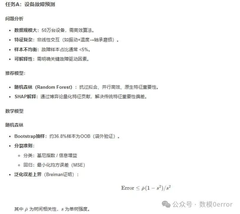
初赛任务A：机床设备故障预测回归分析问题使用机器编号、机器类型、运行小时数、温度、振动、声音、油位、冷却液位、功耗、距

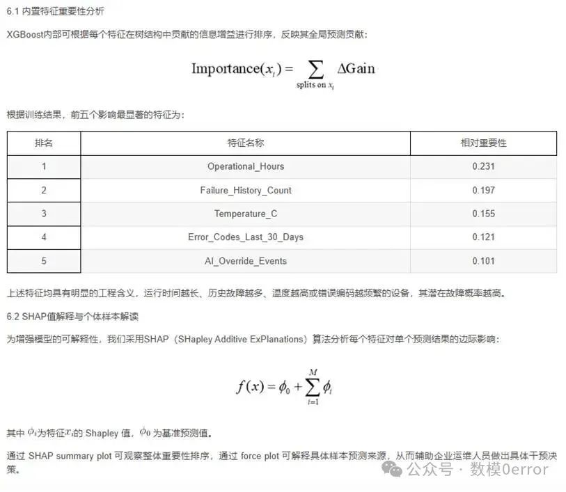
上次维护天数、维护历史次数、故障历史次数、人工智能监控、过去30天错误编码等特征，构建回归模型，预测机床设备在7天内是否会发生故障。要求输出模型准确率、召回率、F1值，并分析前5个最重要的特征。

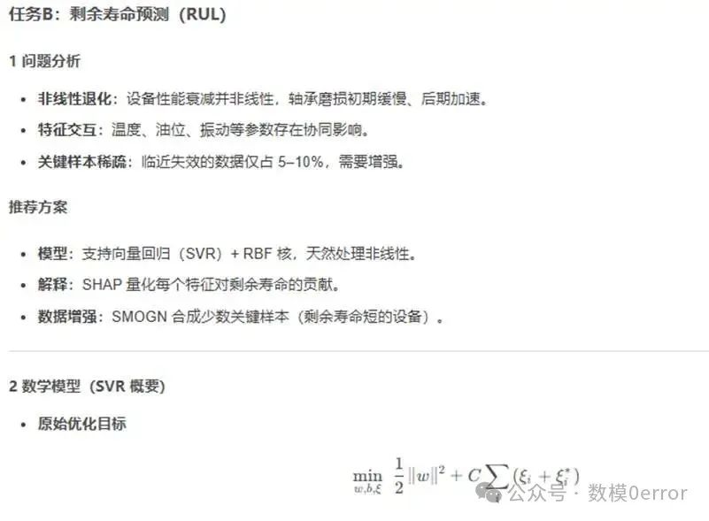
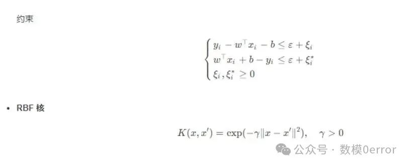
初赛任务B：剩余使用寿命预测回归分析问题

在不使用目标标签（7天内故障预测）的情况下，基于剩余使用寿命（天）、运行小时数、 温度、振动、油位、冷却液位、维护历史次数、故障历史次数等特征，构建回归模型，预测机床设备的剩余使用寿命（目标为连续值）。要求输出模型的均方误差（MSE）和决定系数（R²）并分析特征重要性对剩余寿命的影响。

题目声明：本赛事所有赛题仅授权2025年第四届“创新杯”（原钉钉杯）大学生大数据挑战赛参赛队伍使用，任何组织及个人未经组委会书面授权，严禁用于校内竞赛，篡改、复制等侵权行为。

import pandas as pd

import numpy as np

from sklearn.ensemble import RandomForestClassifier

from sklearn.metrics import accuracy_score, recall_score, f1_score

from sklearn.preprocessing import StandardScaler, OneHotEncoder

from imblearn.over_sampling import SMOTE

import shap

# 数据加载与预处理

data = pd.read_csv('sensor_data.csv')

X = data.drop(['Failure_Within_7_Days', 'Machine_ID'], axis=1)

y = data['Failure_Within_7_Days']

# 类别特征编码

encoder = OneHotEncoder(sparse_output=False)

encoded_cols = encoder.fit_transform(X[['Machine_Type']])

X_encoded = pd.concat([X.drop('Machine_Type', axis=1), pd.DataFrame(encoded_cols)], axis=1)

# 标准化连续特征

scaler = StandardScaler()

cont_features = ['Temperature_C', 'Vibration_mms', 'Operational_Hours']

X_encoded[cont_features] = scaler.fit_transform(X_encoded[cont_features])

# SMOTE过采样（若故障样本<5%）

if sum(y) / len(y) < 0.05:

 smote = SMOTE(random_state=42)

 X_res, y_res = smote.fit_resample(X_encoded, y)

else:

 X_res, y_res = X_encoded, y

# 划分训练集与测试集

X_train, X_test, y_train, y_test = train_test_split(X_res, y_res, test_size=0.2, random_state=42)

# 训练随机森林

model = RandomForestClassifier(n_estimators=200, max_depth=10, class_weight='balanced', random_state=42)

model.fit(X_train, y_train)

# 预测与评估

y_pred = model.predict(X_test)

print("Accuracy:", accuracy_score(y_test, y_pred))

print("Recall:", recall_score(y_test, y_pred))

print("F1 Score:", f1_score(y_test, y_pred))

# SHAP特征重要性分析

explainer = shap.TreeExplainer(model)

shap_values = explainer.shap_values(X_test)

shap.summary_plot(shap_values[1], X_test, plot_type="bar")

import pandas as pd

import numpy as np

from sklearn.svm import SVR

from sklearn.preprocessing import StandardScaler

from sklearn.metrics import mean_squared_error, r2_score

from sklearn.model_selection import train_test_split, GridSearchCV

import shap

import smogn# SMOGN: 针对回归的少数样本合成

# 1. 读取数据

data = pd.read_csv('sensor_data.csv')

# 2. 特征与标签

features = ['Operational_Hours', 'Temperature_C', 'Vibration_mms',

'Oil_Level_pct', 'Coolant_Level_pct', 'Maintenance_History_Count']

X = data[features]

y = data['Remaining_Useful_Life_days']

# 3. 关键样本增强（SMOGN）

low_life = np.percentile(y, 10)

X_res, y_res = smogn.smoter(

data=pd.concat([X, y], axis=1),

y='Remaining_Useful_Life_days',

pert=0.05,

y_thresh=low_life

)

# 4. 标准化

X_scaler = StandardScaler()

y_scaler = StandardScaler()

X_scaled = X_scaler.fit_transform(X_res)

y_scaled = y_scaler.fit_transform(y_res.values.reshape(-1, 1)).ravel()

# 5. 训练/测试划分

X_train, X_test, y_train, y_test = train_test_split(

X_scaled, y_scaled, test_size=0.2, random_state=42)

# 6. 网格搜索最优超参数

param_grid = {

'C':      [0.1, 1, 10, 100],

'gamma':  [0.01, 0.1, 1],

'epsilon':[0.05, 0.1, 0.2]

}

svr = SVR(kernel='rbf')

grid = GridSearchCV(svr, param_grid, cv=5,

scoring=['neg_mean_squared_error','r2'],

refit='neg_mean_squared_error',

 n_jobs=-1)

grid.fit(X_train, y_train)

best = grid.best_estimator_

# 7. 预测与反标准化

y_pred_scaled = best.predict(X_test)

y_pred = y_scaler.inverse_transform(y_pred_scaled.reshape(-1, 1)).ravel()

y_test_orig = y_scaler.inverse_transform(y_test.reshape(-1, 1)).ravel()

# 8. 评估指标

mse = mean_squared_error(y_test_orig, y_pred)

r2 = r2_score(y_test_orig, y_pred)

print(f"MSE = {mse:.2f}, R² = {r2:.4f}")

# 9. SHAP 解释

explainer = shap.KernelExplainer(best.predict,

shap.sample(X_train, 100))

shap_values = explainer.shap_values(X_test)

# 9.1 全局特征重要性

shap.summary_plot(shap_values, X_test,

feature

# 1. 导入必要库

import pandas as pd

import numpy as np

import matplotlib.pyplot as plt

import seaborn as sns

from sklearn.model_selection import train_test_split, GridSearchCV

from sklearn.preprocessing import StandardScaler

from sklearn.impute import SimpleImputer

from sklearn.utils import class_weight

from sklearn.metrics import classification_report, confusion_matrix, accuracy_score, recall_score, f1_score

from xgboost import XGBClassifier, plot_importance

# import shap# 如果你本地支持，可启用此行

# 2. 读取数据

df = pd.read_csv("train_data.csv")

# 3. 初步处理

df['AI_Supervision'] = df['AI_Supervision'].astype(int)

df['Failure_Within_7_Days'] = df['Failure_Within_7_Days'].astype(int)

# 4. 删除缺失值超过80%的列

missing_ratio = df.isnull().mean()

df = df.loc[:, missing_ratio < 0.8]

# 5. 衍生新特征

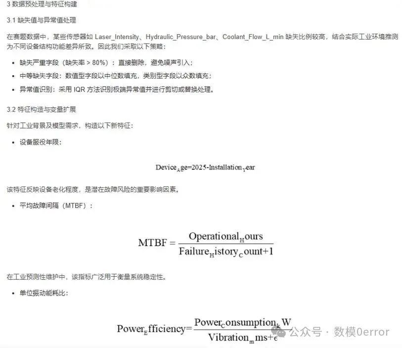
df['Device_Age'] = 2025 - df['Installation_Year']

df['MTBF'] = df['Operational_Hours'] / (df['Failure_History_Count'] + 1)

df['Power_Efficiency'] = df['Power_Consumption_kW'] / (df['Vibration_mms'] + 1e-5)

# 6. 删除无用列

df = df.drop(columns=['Machine_ID', 'Installation_Year'])

# 7. 类别变量独热编码

df = pd.get_dummies(df, columns=['Machine_Type'], drop_first=True)

# 8. 分离特征和标签

X = df.drop(columns=['Failure_Within_7_Days'])

y = df['Failure_Within_7_Days']

# 9. 缺失值填补

imputer = SimpleImputer(strategy='median')

X_imputed = imputer.fit_transform(X)

# 10. 特征标准化

scaler = StandardScaler()

X_scaled = scaler.fit_transform(X_imputed)

# 11. 划分训练集和测试集

X_train, X_test, y_train, y_test = train_test_split(X_scaled, y, stratify=y, test_size=0.2, random_state=42)

# 12. 样本权重处理

weights = class_weight.compute_sample_weight(class_weight='balanced', y=y_train)

# 13. 建立并训练XGBoost模型

model = XGBClassifier(

learning_rate=0.1,

n_estimators=100,

max_depth=6,

subsample=0.8,

colsample_bytree=0.8,

random_state=42,

use_label_encoder=False,

eval_metric='logloss'

)

model.fit(X_train, y_train, sample_weight=weights)

# 14. 模型预测与评估

y_pred = model.predict(X_test)

print("准确率 Accuracy:", accuracy_score(y_test, y_pred))

print("召回率 Recall:", recall_score(y_test, y_pred))

print("F1值 F1 Score:", f1_score(y_test, y_pred))

print("\n分类报告 Classification Report:\n", classification_report(y_test, y_pred))

# 15. 混淆矩阵可视化

cm = confusion_matrix(y_test, y_pred)

plt.figure(figsize=(6, 5))

sns.heatmap(cm, annot=True, fmt='d', cmap='Blues')

plt.title("Confusion Matrix")

plt.xlabel("Predicted")

plt.ylabel("Actual")

plt.tight_layout()

plt.show()

# 16. 特征重要性可视化

plt.figure(figsize=(10, 6))

plot_importance(model, max_num_features=10)

plt.title("Top 10 Important Features (XGBoost)")

plt.tight_layout()

plt.show()

# 17. 可选：SHAP值解释（需在本地安装支持的llvmlite和shap库）

# explainer = shap.Explainer(model)

# shap_values = explainer(X_test)

# shap.summary_plot(shap_values, features=X_test, feature_names=X.columns)

通过网盘分享的文件：2025钉钉杯（创新杯）资料
链接: https://pan.baidu.com/s/1IPfcDObvPTCtjVx4UbTl3Q 提取码: yutf