和前面体光子晶体一样，代码也是从Photonic Crystals Physics and Practical Modeling (Igor A. Sukhoivanov, Igor V. Guryev 这本书上扒下来的(page 197)

这个代码同样用的数值法算的相对介电函数的傅里叶系数

书上的原始代码似乎有些问题，它的结果和FEM的结果符合得不是很好

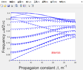
原始代码为：

function PhC_waveguide
%The program for the computation of the dispersion
%characteristic of the PhC waveguide based upon 2D
%PhC with square latice. Parameters of the structure
%are defined by the PhC period, elements radius, and
%by the permittivities of elements and background
%material. In contrast to pure PhC, the waveguide is
%also defined by the number or the elements in
%direction transversal to radiation propagation as
%well as by the number of elements missed to form
%the defect.
%Main part of the program is implemented as a
%function because it should be run two times, namely,
%for the structure with and without defect. At first
%run, the function computes the defect eigen-states
%and at the first run it compute the continuum of
%states of the PhC.
%Input parameters: PhC period, radius of an
%element, permittivities, number of elements in
%transversal direction, defect size
%Output data: The dispersion diagram of the
%2D PhC waveguide.
clear ;close all
%The variable a defines the period of the structure.
%It influences on results in case of the frequency
%normalization.
a=1e-6;%晶格常数
%The variable r contains elements radius. Here it is
%defined as a part of the period.
r=0.4*a;%圆柱半径
%The variable eps1 contains the information about
%the relative background material permittivity.
eps1=9;%背景的相对介电常数
%The variable eps2 contains the information about
%permittivity of the elements composing PhC. In our
%case permittivities are set to form the structure
%perforated membrane
eps2=1;%柱子的相对介电常数
%Variable numElem defines the number of PhC elements
%in direction transversal to radiation propagation
numElem=7;%条状超原胞大小
%Number of holes missed
numDef=1;%缺陷大小
%Setting transversal wave vector to a single value
kx=0;
%Callint the function to copmpute the defect
%eigen-states. With this, we obtain the eigen-states
%of the linear defect
PWE(a, r, eps1, eps2, numElem, numDef, kx, "b", 1);
numElem=1;%条状超原胞大小
numDef=0;%缺陷大小
%Setting transversal wave vector to a range of
%values within Brillouin zone
kx=0:(pi/a)/200:pi/a;%设定的值要在布里渊区内
%Callint the function to copmpute the eigen-states
%of bulk PhC. This action fills the area of the
%continuum of states giving the possibility to
%analize the dispersion diagram

PWE(a, r, eps1, eps2, numElem, numDef, kx, 'r', 3);


function PWE(a, r, eps1, eps2, numElem,...
    numDefect, kx_param, color, linewidth)
%The function implements the PWE method for 2D PhC
%The inputs are structure geometry and parameters,
%the number of transversal elements of the waveguide,
%the number of holed missed to form the defect and
%the transversal wave vectors set
%Computation precision parameters are set inside the
%function
%The variable precis defines the number of k-vector
%points between high symmetry points
precis=29;%高对称点间布里渊区的离散点数

%The variable nG defines the number of plane waves.
%Since the number of plane waves cannot be
%arbitrary value and should be zero-symmetric, the
%total number of plane waves may be determined
%as (nG*2-1)^2
nG=8;%定义了平面波的数量
%The variable precisStruct defines contains the
%number of nodes of discretization mesh inside in
%unit cell
%discretization mesh elements.
precisStruct=30;%定义了单位原胞内离散网格的节点数
%The following loop carries out the definition
%of the unit cell. The definition is being
%made in discreet form by setting values of inversed
%dielectric function to mesh nodes.
for n=0:numElem-1
    nx=1;
    for countX=-a/2:a/precisStruct:a/2
        ny=1;
        for countY=-a/2:a/precisStruct:a/2
            %Following condition allows to define the circle
            %with of radius r
            if((sqrt(countX^2+countY^2)<r)&&(n>=numDefect))
                %Setting the value of the inversed dielectric
                %function to the mesh node
                struct(nx+precisStruct*n,ny)=1/eps2;
                %Saving the node coordinate
                xSet(nx+precisStruct*n)=countX+a*n;
                ySet(ny)=countY;
            else
                struct(nx+precisStruct*n,ny)=1/eps1;
                xSet(nx+precisStruct*n)=countX+a*n;
                ySet(ny)=countY;
            end
            ny=ny+1;
        end
        nx=nx+1;
    end
end
%The computation of the area of the mesh cell. It is
%necessary for further computation of the Fourier
%expansion coefficients.
dS=(a/precisStruct)^2;
%Forming 2D arrays of nods coordinates
[xMesh, yMesh]=meshgrid(xSet(1:length(xSet)),...
    ySet(1:length(ySet)));
%Transforming values of inversed dielectric function
%for the convenience of further computation
structMesh=(struct(1:length(xSet),1:length(ySet))*...
    dS/((max(xSet)-min(xSet))*(max(ySet)-min(ySet))))';
b1=[2*pi/a 0]./numElem;
b2=[0 2*pi/a];


%Defining the k-path within the Brilluoin zone. The
%k-path includes all high symmetry points and precis
%points between them
kx0(1:precis+1)=zeros(1,precis+1);
ky(1:precis+1)=0:b2(2)/2/precis:b2(2)/2;
%After the following loop, the variable numG will
%contain real number of plane waves used in the
%Fourier expansion
numG=1;
for Gx=-nG*numElem:nG*numElem%Gx  Gy都是整数
    for Gy=-nG:nG
        G(numG,1:2)=Gx.*b1+Gy.*b2;
        
        numG=numG+1;
    end
end
%The next loop computes the Fourier expansion
%coefficients which will be used for matrix
%differential operator computation.
for countG=1:numG-1
    for countG1=1:numG-1
        CN2D_N(countG,countG1)=sum(sum(structMesh.*...
            exp(-1i*((G(countG,1)-G(countG1,1))*xMesh+...
            (G(countG,2)-G(countG1,2))*yMesh))));
    end
end



%The next loop computes matrix differential
%operator in case of TE mode. The computation
%is carried out for each of earlier defined
%wave vectors.
for kx_count=1:length(kx_param)
    kx=kx0+kx_param(kx_count);
    for countG=1:numG-1
        for countG1=1:numG-1
            for countK=1:length(kx)
                M(countK,countG,countG1)=...
                    CN2D_N(countG,countG1)*...
                    ((kx(countK)+G(countG,1))*...
                    (kx(countK)+G(countG1,1))+...
                    (ky(countK)+G(countG,2))*...
                    (ky(countK)+G(countG1,2)));
            end
        end
    end
    %The computation of eigen-states is also carried
    %out for all wave vectors in the k-path.
    
    for countK=1:length(kx)
        %Taking the matrix differential operator for
        %current wave vector.
        MM(:,:)=M(countK,:,:);
        %Computing the eigen-vectors and eigen-states of
        %the matrix
        [D,V]=eig(MM);
        %Transforming matrix eigen-states to the form of
        %normalized frequency.
        dispe(:,countK)=sort((sqrt(V*...
            ones(length(V),1)))*a/2/pi);
    end
    figure(1);
    hold on;
    for u=1:15
        plot(ky,abs(dispe(u,:)),color,...
            'LineWidth',linewidth);
    end
    ylabel('Frequency \omegaa/2\pic','FontSize',20);
    xlabel('Propagaion constant \beta, m^{-1}',...
        'FontSize',20);
    drawnow;
    ylim([0,0.37])
    xlim([0,3*1e6])
end

这个代码相对于书上的代码改了点参数，但其他部分和书上完全一样。

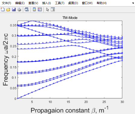
可以看到原始的代码和前面文章体光子晶体的数值算法思想不一样了，刚开始我思考了很久以为哪里没搞明白，但后来我修改了代码并和FEM的结果进行了比较，发现修改后代码得到的结果和FEM更符合，图像如下(蓝线是PWE的结果，蓝色小圆是FEM的结果)：

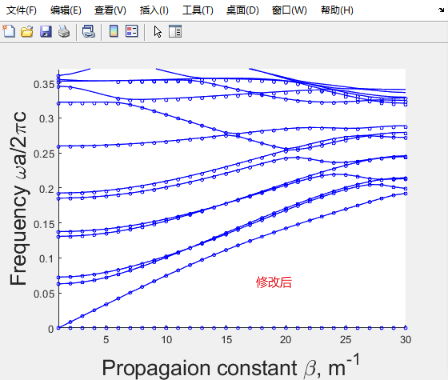
但为了保险我还是发邮件问了作者，不过目前还没回复。(ps:这是09年的书了，不知道作者还会不会回复)

修改后的代码：

function PhC_waveguide_Test
%The program for the computation of the dispersion
%characteristic of the PhC waveguide based upon 2D
%PhC with square latice. Parameters of the structure
%are defined by the PhC period, elements radius, and
%by the permittivities of elements and background
%material. In contrast to pure PhC, the waveguide is
%also defined by the number or the elements in
%direction transversal to radiation propagation as
%well as by the number of elements missed to form
%the defect.
%Main part of the program is implemented as a
%function because it should be run two times, namely,
%for the structure with and without defect. At first
%run, the function computes the defect eigen-states
%and at the first run it compute the continuum of
%states of the PhC.
%Input parameters: PhC period, radius of an
%element, permittivities, number of elements in
%transversal direction, defect size
%Output data: The dispersion diagram of the
%2D PhC waveguide.
clear ;close all;clc
%The variable a defines the period of the structure.
%It influences on results in case of the frequency
%normalization.
a=1e-6;%晶格常数
%The variable r contains elements radius. Here it is
%defined as a part of the period.
r=0.4*a;%圆柱半径
%The variable eps1 contains the information about
%the relative background material permittivity.
eps1=9;%背景的相对介电常数
%The variable eps2 contains the information about
%permittivity of the elements composing PhC. In our
%case permittivities are set to form the structure
%perforated membrane
eps2=1;%柱子的相对介电常数
%Variable numElem defines the number of PhC elements
%in direction transversal to radiation propagation
numElem=7;%条状超原胞大小
%Number of holes missed
numDef=1;%缺陷大小
%Setting transversal wave vector to a single value
kx=0;
%Callint the function to copmpute the defect
%eigen-states. With this, we obtain the eigen-states
%of the linear defect
PWE(a, r, eps1, eps2, numElem, numDef, kx, "b", 1);
numElem=1;%条状超原胞大小
numDef=0;%缺陷大小
%Setting transversal wave vector to a range of
%values within Brillouin zone
kx=0:(pi/a)/200:pi/a;%设定的值要在布里渊区内
%Callint the function to copmpute the eigen-states
%of bulk PhC. This action fills the area of the
%continuum of states giving the possibility to
%analize the dispersion diagram

%PWE(a, r, eps1, eps2, numElem, numDef, kx, 'r', 3);%这部分将会绘制很多很密的线条


function PWE(a, r, eps1, eps2, numElem,...
    numDefect, kx_param, color, linewidth)
%The function implements the PWE method for 2D PhC
%The inputs are structure geometry and parameters,
%the number of transversal elements of the waveguide,
%the number of holed missed to form the defect and
%the transversal wave vectors set
%Computation precision parameters are set inside the
%function
%The variable precis defines the number of k-vector
%points between high symmetry points
precis=29;%高对称点间布里渊区的离散点数

%The variable nG defines the number of plane waves.
%Since the number of plane waves cannot be
%arbitrary value and should be zero-symmetric, the
%total number of plane waves may be determined
%as (nG*2-1)^2
nG=8;%定义了平面波的数量
%The variable precisStruct defines contains the
%number of nodes of discretization mesh inside in
%unit cell
%discretization mesh elements.
precisStruct=30;%定义了单位原胞内离散份数
%The following loop carries out the definition
%of the unit cell. The definition is being
%made in discreet form by setting values of inversed
%dielectric function to mesh nodes.
for n=0:numElem-1%0~6
    nx=1;
    for countX=-a/2:a/precisStruct:a/2
        ny=1;
        for countY=-a/2:a/precisStruct:a/2
            %Following condition allows to define the circle
            %with of radius r
            if((sqrt(countX^2+countY^2)<r)&&(n>=numDefect))%这里numDefect=1
                %Setting the value of the inversed dielectric
                %function to the mesh node
                struct(nx+precisStruct*n,ny)=1/eps2;
                %Saving the node coordinate
                xSet(nx+precisStruct*n)=countX+a*n;
                ySet(ny)=countY;
            else
                struct(nx+precisStruct*n,ny)=1/eps1;
                xSet(nx+precisStruct*n)=countX+a*n;
                ySet(ny)=countY;
            end
            ny=ny+1;
        end
        nx=nx+1;
    end
end
size(struct);%211 31

figure
mesh(struct)
axis equal
%The computation of the area of the mesh cell. It is
%necessary for further computation of the Fourier
%expansion coefficients.
dS=(a/precisStruct)^2;
%Forming 2D arrays of nods coordinates
[xMesh, yMesh]=meshgrid(xSet(1:length(xSet)),...
    ySet(1:length(ySet)));
%======================%
xMesh(:,end)=[];
xMesh(end,:)=[];
yMesh(:,end)=[];
yMesh(end,:)=[];
%======================%

% figure
% for ii = 1:numel(xMesh)
%     plot(xMesh(ii),yMesh(ii),'b.','Markersize',10)
%     hold on
%     
%     %rectangle('Position',[xMesh(ii),...
%         %yMesh(ii),(a/precisStruct),(a/precisStruct)]);
%     
% end
% axis equal


size(xMesh);%31   211
size(yMesh);%31   211
length(xSet);%211
%Transforming values of inversed dielectric function
%for the convenience of further computation
%====================================%
structMesh=(struct(1:length(xSet)-1,1:length(ySet)-1)*...
    dS/((max(xSet)-min(xSet))*(max(ySet)-min(ySet))))';
%====================================%

b1=[2*pi/a 0]./numElem;
b2=[0 2*pi/a];
%横着的条状超原胞，宽numElem*a，高a


(max(xSet)-min(xSet))./a;%7
(max(ySet)-min(ySet))./a;%1
size(struct);% 211*31
size(structMesh);%31*211


%Defining the k-path within the Brilluoin zone. The
%k-path includes all high symmetry points and precis
%points between them
kx0(1:precis+1)=zeros(1,precis+1);
ky(1:precis+1)=0:b2(2)/2/precis:b2(2)/2;%布里渊区似乎只考虑了一条线上的(0~pi/a)
%ky长度30

%After the following loop, the variable numG will
%contain real number of plane waves used in the
%Fourier expansion

numG=1;
for Gx=-nG*numElem:nG*numElem%Gx  Gy都是整数
    for Gy=-nG:nG
        G(numG,1:2)=Gx.*b1+Gy.*b2;
        
        numG=numG+1;
    end
end
%The next loop computes the Fourier expansion
%coefficients which will be used for matrix
%differential operator computation.
for countG=1:numG-1
    mark0=countG/(numG-1)
    for countG1=1:numG-1
        CN2D_N(countG,countG1)=sum(sum(structMesh.*...
            exp(-1i*((G(countG,1)-G(countG1,1))*xMesh+...
            (G(countG,2)-G(countG1,2))*yMesh))));
    end
end
size(CN2D_N);%145*145



%The next loop computes matrix differential
%operator in case of TE mode. The computation
%is carried out for each of earlier defined
%wave vectors.
for kx_count=1:length(kx_param)
    kx=kx0+kx_param(kx_count);
    for countG=1:numG-1
        countG/(numG-1)
        for countG1=1:numG-1
            for countK=1:length(kx)
                M(countK,countG,countG1)=...
                    CN2D_N(countG,countG1)*...
                    ((kx(countK)+G(countG,1))*...
                    (kx(countK)+G(countG1,1))+...
                    (ky(countK)+G(countG,2))*...
                    (ky(countK)+G(countG1,2)));
            end
        end
    end
    %The computation of eigen-states is also carried
    %out for all wave vectors in the k-path.
    
    for countK=1:length(kx)
        Mark=countK/length(kx)
        %Taking the matrix differential operator for
        %current wave vector.
        MM(:,:)=M(countK,:,:);
        %Computing the eigen-vectors and eigen-states of
        %the matrix
        [D,V]=eig(MM);
        %Transforming matrix eigen-states to the form of
        %normalized frequency.
        dispe(:,countK)=sort((sqrt(V*...
            ones(length(V),1)))*a/2/pi);
    end
    figure
    hold on;
    for u=1:15
        plot(1:length(ky),abs(dispe(u,:)),color,...
            'LineWidth',linewidth);
    end
    hold on
    %下面是和FEM算的数据比较，没有的话可以删除下面这段%%

Data=csvread('C:\Users\LUO1\Desktop\WaveGuideTE.csv');
uniX=unique(Data(:,1));
Ymat=[];
for zz=1:length(uniX)
    Ymat=[Ymat,Data(Data(:,1)==uniX(zz),2)];
end

plot(1:size(Ymat,2),Ymat,'bo','MarkerSize',3)
hold off
%%%%%绘制FEM的数据%%%%%%%
    
    
    ylabel('Frequency \omegaa/2\pic','FontSize',20);
    xlabel('Propagaion constant \beta, m^{-1}',...
        'FontSize',20);
    drawnow;%好像是动画？
    ylim([0,0.37])
    xlim([1,length(ky)])
end

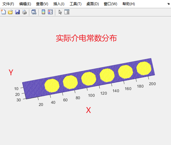
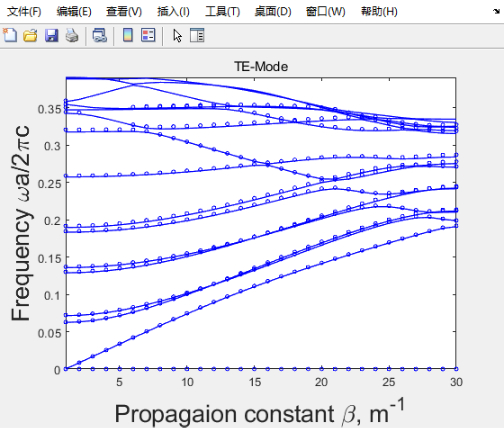
下面我扩展了下前面改进的代码，可以计算TE TM模式，可以计算x或y是长边的超原胞的投影能带

clear ;close all;clc

a=1e-6;%晶格常数

r=0.4*a;%圆柱半径

eps1=9;%背景的相对介电常数

eps2=1;%柱子的相对介电常数
TEorTM='TM';%设置模式

precis=29;%高对称点间布里渊区的离散点数


nG=14;%定义了平面波的数量

precisStruct=30;%定义了正方形单位原胞的离散份数(最好设置为偶数)

unitSto=[0,ones(1,6)];%和正空间条状原胞的结构有关。为0代表没有圆柱，为1代表有圆柱
numElem=length(unitSto);%长边方向的正空间超原胞大小，单位为a(晶格常数)，注意短边方向的numElem永远为1
XorYlong='X';%光子晶体波导正空间原胞X方向还是Y方向是长边。
NumBand=15;%能带绘制条数(归一化频率freq从低到高数)

%%%正空间基矢(需自己设置)%%%
a1=[numElem*a,0,0];%为方便求倒格子基矢，必须是三维矢量
a2=[0,a,0];
%横着的条状超原胞，宽numElem*a，高a
%%%正空间基矢(需自己设置)%%%

%==========计算倒格子基矢==============%
a3=[0,0,1];%单位向量
Omega=abs(a3*cross(a1,a2)');%正空间单位原胞面积
s=2*pi./Omega;
b1(1,1)=a2(1,2);b1(1,2)=-a2(1,1);
b2(1,1)=-a1(1,2);b2(1,2)=a1(1,1);
b1=b1.*s;%1*2行数组，最终结果(必须是行数组)
b2=b2.*s;%1*2行数组，最终结果(必须是行数组)
%==========计算倒格子基矢==============%



unitX=-a/2:a/precisStruct:a/2;%一个长宽都是a坐标中心为(0,0)的正空间单位原胞的离散网格节点的x坐标
unitY=unitX;%同上，但是是y坐标
lenNode=length(unitX);

if strcmp(XorYlong,'X')==1
    struct=zeros(precisStruct+1,precisStruct*numElem+1);
    Mesh=zeros(precisStruct+1,precisStruct*numElem+1);
    Lx=numElem*a;
    Ly=a;
end

if strcmp(XorYlong,'Y')==1
    struct=zeros(precisStruct*numElem+1,precisStruct+1);
    Mesh=zeros(precisStruct*numElem+1,precisStruct+1);
    Lx=a;
    Ly=numElem*a;
end



for n=0:numElem-1
    if strcmp(XorYlong,'X')==1
        
        for nx=1:lenNode%precisStruct+1个数据，变nx，nx=1~precisStruct+1
            countX=unitX(nx);
            for ny=1:lenNode%变ny，ny=1~precisStruct+1
                countY=unitY(ny);
                
                if abs(countX+1j*countY)<r && unitSto(n+1)==1
                    struct(ny,nx+precisStruct*n)=1/eps2;%柱子的相对介电常数
                    Mesh(ny,nx+precisStruct*n)=(countX+a*n)+1j*countY;%节点坐标
                    
                else
                    struct(ny,nx+precisStruct*n)=1/eps1;%背景的相对介电常数
                    Mesh(ny,nx+precisStruct*n)=(countX+a*n)+1j*countY;%节点坐标
                    
                end
            end
        end
        
    end
    %==================================%
    
    if strcmp(XorYlong,'Y')==1
        
        for nx=1:lenNode%precisStruct+1个数据，变nx，nx=1~precisStruct+1
            countX=unitX(nx);
            for ny=1:lenNode%变ny，ny=1~precisStruct+1
                countY=-unitY(ny);
                
                if abs(countX+1j*countY)<r && unitSto(n+1)==1
                    struct(ny+precisStruct*n,nx)=1/eps2;%柱子的相对介电常数
                    Mesh(ny+precisStruct*n,nx)=countX+1j*(countY-a*n);%节点坐标
                else
                    struct(ny+precisStruct*n,nx)=1/eps1;%背景的相对介电常数
                    Mesh(ny+precisStruct*n,nx)=countX+1j*(countY-a*n);%节点坐标
                end
                
            end
        end
        
    end
    
    %struct元素要和xMesh、yMesh元素位置相匹配
end

xMesh=real(Mesh);
yMesh=imag(Mesh);
%xMesh是所有节点的x坐标；yMesh是所有节点的y坐标
%xMesh、yMesh合起来其实相当于存储了所有节点的坐标
%=====================%
%=====================%
figure
imagesc(1./struct);
colorbar;
colormap(jet);
axis equal
xlabel('X')
ylabel('Y')
title('相对介电常数分布可视化')
%=====================%
figure
scatter(xMesh(:),yMesh(:),20,'b.')
hold on
scatter(0,0,80,'r.')%绘制坐标原点
hold off
xlabel('X')
ylabel('Y')
axis equal
title('所有节点坐标可视化')
%=====================%
%=====================%


if strcmp(XorYlong,'X')==1
    %下面是删掉部分节点
    xMesh(:,end)=[];
    xMesh(end,:)=[];
    yMesh(:,end)=[];
    yMesh(end,:)=[];
    struct(:,end)=[];
    struct(end,:)=[];
end

if strcmp(XorYlong,'Y')==1
    %下面是删掉部分节点
    xMesh(1,:)=[];
    xMesh(:,end)=[];
    yMesh(1,:)=[];
    yMesh(:,end)=[];
    struct(1,:)=[];
    struct(:,end)=[];
end


dS=(a/precisStruct)^2;
structMesh=(dS/(Lx*Ly)).*struct;


% figure
% for ii = 1:numel(xMesh)
%     plot(xMesh(ii),yMesh(ii),'b.','Markersize',10)
%     hold on
%
%     %rectangle('Position',[xMesh(ii),...
%         %yMesh(ii),(a/precisStruct),(a/precisStruct)]);
%
% end
% axis equal


%======离散BZ(需要根据实际情况设置)=======%
kx0=zeros(1,precis+1);%行数组
ky0=linspace(0,pi/a,precis+1);%行数组，布里渊区似乎只考虑了一条线上的(0~pi/a)
kx_ky0=kx0+1j.*ky0;

%======离散BZ(需要根据实际情况设置)=======%


numG0=0;
for mm=-nG*numElem:nG*numElem%mm  nn都是整数
    for nn=-nG:nG
        numG0=numG0+1;
        G(numG0,1:2)=mm.*b1+nn.*b2;
        
    end
end
numG=size(G,1);%行

Kap=zeros(numG,numG);
for countG=1:numG
    Kapmark=countG/(numG)
    for countG1=1:numG
        Exp=exp(-1j*((G(countG,1)-G(countG1,1)).*xMesh+...
            (G(countG,2)-G(countG1,2)).*yMesh));%矩阵
        
        Kap(countG,countG1)=sum(sum(structMesh.*Exp));
        %其实就是kappa(G_{||}-G_{||}^{\prime}})构成的矩阵
        %G(countG,1:2)其实就是G_{||}，
        %G(countG1,1:2)其实就是G_{||}^{\prime}
    end
end



if strcmp(TEorTM,'TE')==1%TE模式
    M=zeros(numG,numG,length(kx_ky0));
    
    for countK=1:length(kx_ky0)
        kx=real(kx_ky0(countK));
        ky=imag(kx_ky0(countK));
        
        for countG=1:numG
            %[Gx,Gy]=G(countG,1:2);
            %[Gx',Gy']=G(countG1,1:2);
            for countG1=1:numG
                M(countG,countG1,countK)=...
                    ((kx+G(countG,1))*...
                    (kx+G(countG1,1))+...
                    (ky+G(countG,2))*...
                    (ky+G(countG1,2)))*Kap(countG,countG1);%TE模式特征矩阵
            end
        end
        
    end
    
end


if strcmp(TEorTM,'TM')==1%TM模式
    M=zeros(numG,numG,length(kx_ky0));
    
    for countK=1:length(kx_ky0)
        kx=real(kx_ky0(countK));
        ky=imag(kx_ky0(countK));
        
        for countG=1:numG
            %[Gx,Gy]=G(countG,1:2);
            %[Gx',Gy']=G(countG1,1:2);
            for countG1=1:numG
                M(countG,countG1,countK)=...
                    Kap(countG,countG1)*...
                    (norm([kx+G(countG,1),ky+G(countG,2)])*...
                    norm([kx+G(countG1,1),ky+G(countG1,2)]));%TM模式特征矩阵
            end
        end
        
    end
    
end



Eigsto=zeros(numG,length(kx_ky0));
for countK=1:length(kx_ky0)
    EigMark=countK/length(kx_ky0)
    
    MM(:,:)=M(:,:,countK);
    
    [vec,val]=eig(MM);
    val=diag(val);%列数组
    freq=sqrt(val)*a/(2*pi);%wa/(2pi c)，归一化频率
    freq=sort(freq);%排序
    Eigsto(:,countK)=freq;
    
end

figure
plot(1:length(kx_ky0),abs(Eigsto(1:NumBand,:)),'b','LineWidth',1);
hold on


%下面是和FEM算的数据比较，没有的话可以删除下面这段%%
if strcmp(TEorTM,'TE')==1
    Data=csvread('C:\Users\LUO1\Desktop\WaveGuideTE.csv');
end

if strcmp(TEorTM,'TM')==1
    Data=csvread('C:\Users\LUO1\Desktop\WaveGuideTM.csv');
end

uniX=unique(Data(:,1));
Ymat=[];
for zz=1:length(uniX)
    Ymat=[Ymat,Data(Data(:,1)==uniX(zz),2)];
end
plot(1:size(Ymat,2),Ymat,'bo','MarkerSize',3)
hold off
%%%%%绘制FEM的数据%%%%%%%

if strcmp(TEorTM,'TE')==1
    title('TE-Mode');
end

if strcmp(TEorTM,'TM')==1
    title('TM-Mode');
end

ylabel('Frequency \omegaa/2\pic','FontSize',20);
xlabel('Propagaion constant \beta, m^{-1}',...
    'FontSize',20);
%drawnow;%好像是动画？
ylim([0,0.37])
xlim([1,length(kx_ky0)])

------------------------------------------------2023.8----------------------------------------

无论是体光子晶体或条带光子晶体的Comsol仿真对比文件都在阿里云盘中，读者可以根据合理要求从我这里获得mph文件